How to sum duplicate values ​​in Excel

Summation is a popular arithmetic operation in Excel. Suppose we have a list of goods in a table, and we need to get their total cost. To do this, you need to use the function SUM. Or the company wants to determine the total consumption of electricity for a certain period. Again, you need to summarize these data.

Function SUM can be used not only independently, but also as a component of other functions.

But in some situations, we need to sum up only the values ​​that meet a certain criterion. For example, add exclusively repeating cell contents to each other. In this case, you need to use one of the two functions that will be described later.

Selective summation in Excel

Selective summation is the next step after learning the standard arithmetic operation of adding multiple values. If you learn to read and use it, you can come close to being powerful with Excel. To do this, in the list of Excel formulas, you need to find the following functions.

SUMIF function

Suppose we have such a dataset.

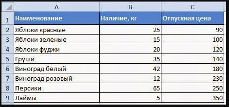
This is a report provided by the vegetable store warehouse. Based on this information, we need to do the following:

1. Determine how much is left in stock for a particular item.
2. Calculate inventory balances along with a price that matches user-defined rules.

Using the function SUMMESLI we can isolate specific meanings and summarize them exclusively. Let’s list the arguments of this operator:

1. Range. This is a set of cells that must be analyzed for compliance with a certain criterion. In this range, there can be not only numeric, but also text values.
2. Condition. This argument specifies the rules by which the data will be selected. For example, only values ​​that match the word “Pear” or numbers greater than 50.
3. summation range. If not needed, you can omit this option. It should be used if a set of text values ​​is used as a range for checking a condition. In this case, you need to specify an additional range with numeric data.

To fulfill the first goal we set, you need to select the cell in which the result of the calculations will be recorded and write the following formula there: =SUMIF(A2:A9;”White grapes”;B2:B9).

The result will be a value of 42. If we had several cells with the value “White Grapes”, then the formula would return the total of the sum of all the positions of this plan.

SUM function

Now let’s try to deal with the second problem. Its main difficulty is that we have several criteria that the range must meet. To solve it, you need to use the function SUMMESLIMN, whose syntax includes the following arguments:

1. summation range. Here this argument means the same as in the previous example.
2. Condition range 1 is a set of cells in which to select those that meet the criteria described in the argument below.
3. Condition 1. Rule for the previous argument. The function will select only those cells from range 1 that match condition 1.
4. Condition range 2, condition 2, and so on.

Further, the arguments are repeated, you just need to sequentially enter each next range of the condition and the criterion itself. Now let’s start solving the problem.

Suppose we need to determine what is the total weight of apples left in the warehouse, which cost more than 100 rubles. To do this, write the following formula in the cell in which the final result should be: =СУММЕСЛИМН(B2:B9;A2:A9;»яблоки*»;C2:C9;»>100″)

In simple words, we leave the summation range the same as it was. After that, we prescribe the first condition and the range for it. After that, we set the requirement that the price should be more than 100 rubles.

Notice the asterisk (*) as the search term. It indicates that any other values ​​can follow it.

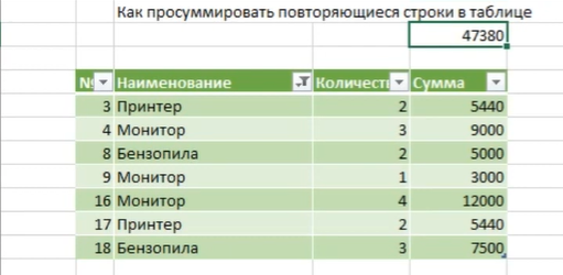
How to sum duplicate rows in a table using smart table

Suppose we have such a table. It was made using the Smart Table tool. In it, we can see duplicate values ​​placed in different cells.

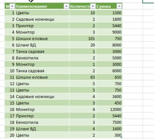
The third column lists the prices of these items. Let’s say we want to know how much repetitive products will cost in total. What do I need to do? First you need to copy all the duplicate data to another column.

After that, you need to go to the “Data” tab and click on the “Delete Duplicates” button.

After that, a dialog box will appear in which you need to confirm the removal of duplicate values.

Special Paste Conversion

Then we will be left with a list of only those values ​​that do not repeat.

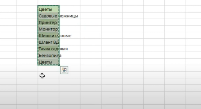
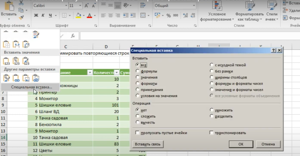
We need to copy them and go to the “Home” tab. There you need to open the menu located under the “Insert” button. To do this, click on the arrow, and in the list that appears, we find the item “Paste Special”. A dialog box like this will appear.

Transposing row to columns

Check the box next to “Transpose” and click OK. This item swaps columns and rows. After that, we write in an arbitrary cell the function SUMMESLI.

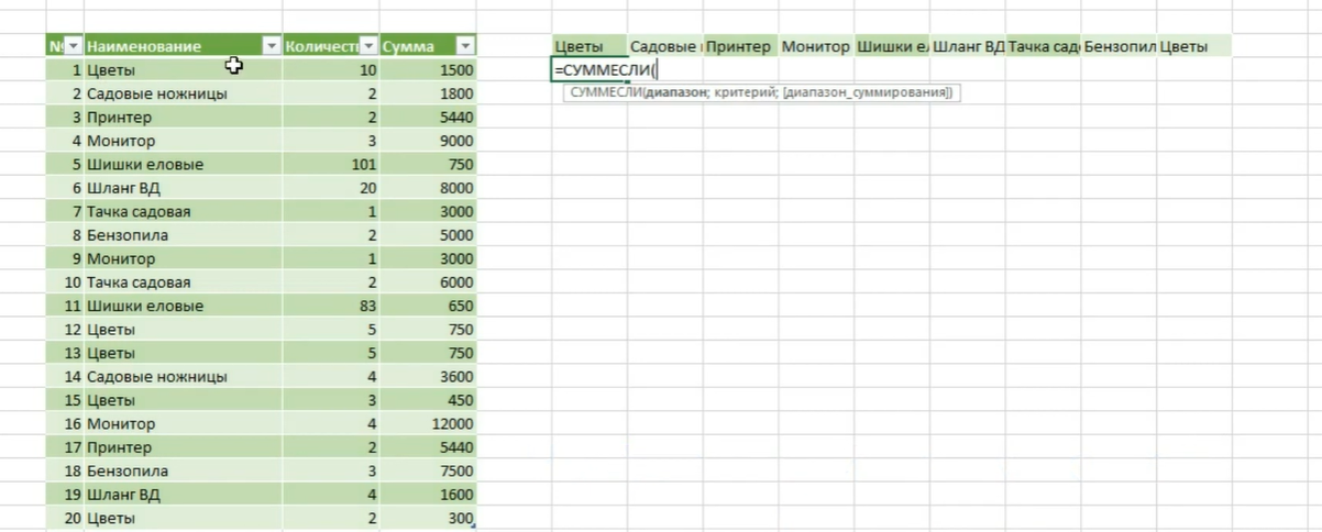
The formula in our case will look like this.

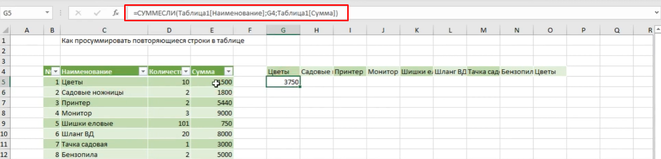
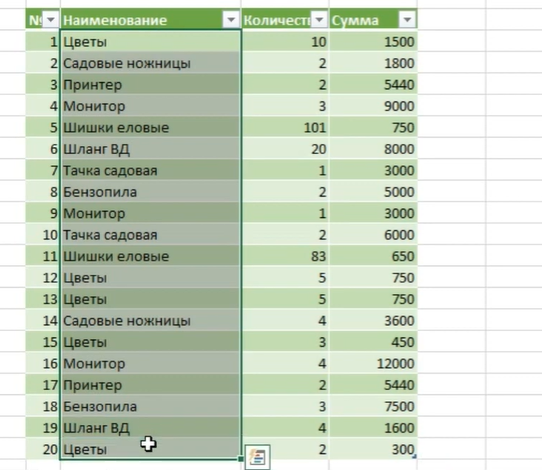
Then, using the autofill marker, fill in the remaining cells. You can also use the function SUBTOTALS in order to summarize the table values. But you must first set a filter for the smart table so that the function counts only repeating values. To do this, click on the arrow icon in the column header, and then check the boxes next to those values ​​that you want to show.

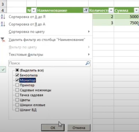
After that, we confirm our actions by pressing the OK button. If we add another item to display, we will see that the total amount will change.

As you can see, you can perform any task in Excel in several ways. You can choose the ones that are suitable for a particular situation or just use the tools that you like best.