How to freeze a row in Excel 2003 on scroll

Many Excel users wonder how an area is fixed in Microsoft Excel. Often there is no intuitive answer to this question, since the corresponding button is not located in the “Home” section. And the number of buttons is too large, and finding the right one among all this variety is not very easy. Therefore, many novice Excel users scroll the table repeatedly.

If the number of lines is small, then there should be no problems. But what if there are a lot of rows in our table, up to a thousand? After all, it is very inconvenient when you have to scroll to the very beginning of a whole list of hundreds of items just to see the name of the desired column. And in the process, you can easily lose the understanding of which row you have worked with before. You can, of course, remember, but even here there is a high probability of simply forgetting.

To avoid all the described problems, it is necessary to use a special function that makes it possible to make one or more of the top rows fixed, and they will not be able to scroll at the same time as the rest. Today we will analyze what needs to be done for this in different versions of Microsoft Excel.

How to make a fixed table header in Excel 2003, 2007 and 2010

Excel was developed in such a way that it would be more convenient for the user not only to analyze data automatically, use formulas, but also to carry out simpler manual processing of information. In particular, with the help of the possibility that we are now considering. Freezing one or more top rows or left columns is a very useful feature. Everyone should know how to use it. It has many advantages:

1. Saving time. Constantly scrolling through large amounts of data requires additional time. If there is too much information, then more time is needed.
2. Economy of forces. Going through a huge amount of the same information over and over again requires a lot of effort. Therefore, a person who tries to work like this gets tired very quickly. Here we see a connection with the other points, because from the fact that there is no strength to work, a person works more slowly. This negative effect is superimposed on the fact that in itself the constant scrolling through a huge Excel spreadsheet many times in order to check with the values ​​​​in the first row or column takes a lot of time.
3. Saving money. A typical situation – while the account manager analyzes the data in the spreadsheet in Excel, the client has passed into the hands of competitors. Consequently, his money also went to rivals. To avoid this situation, you need to save time as much as possible. Without money, the company cannot develop normally. Consequently, it does not introduce innovative technologies that do not help employees save time and effort. And the vicious circle closes.

Therefore, there is no other way out than to master the fixation of a row or column in Excel. What exactly needs to be fixed? First of all, it depends on the table presentation format. Here are some specific situations in which you may need to secure a row:

1. If the first line contains column headings, and the user forgets which column belongs to which item. In this case, pinning a line allows you to immediately see the name and understand what this or that number means.
2. If the first row contains data, by month for many years, starting from the first month five years ago. In this case, you may need to freeze the row in order, for example, to compare current data with the same period several years ago. For example, such a situation may arise when it is necessary to analyze financial statements for a certain period of time or sales data in order to determine their dynamics.

And here are some cases in which you need to fix the column:

1. If horizontal scrolling is required in situations where table block names are contained in columns. That is, the cases are the same, only the table is not located vertically, but horizontally.
2. If you need to compare current information with several similar periods of previous years, so as not to scroll the table for a long time.

Also, there are often situations when it is necessary to fix both rows and columns. This happens much less often, but today we will also figure out how it is possible to do this. All of these versions of the information application have the option of fixing one or more rows at the top. To do this, you need to perform a set of several steps, which we will describe in relation to different versions of Excel.

Step 1

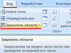
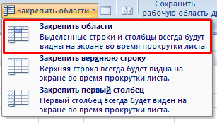
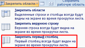
First we need to open the file containing the range where we need to pin one or more top rows. After that, we need to open the “View” menu, and there go to the “Freeze Areas” item. After that, a menu will pop up, where there will be three possible solutions: fix the area, only the top line, or only the first column.

You need to choose the item that is appropriate in a particular situation. If you need to fix only the top row, you need to click on the corresponding button. If it is necessary to fix more than one row, you must click on the “Freeze area” button, after selecting the corresponding rows. We will give a simple example: we only fix the top row. After that, you need to click on it.

Step 2

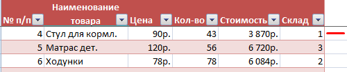
As you can see, the first line is separated from the rest which will scroll. You can understand this by the characteristic black line, which will be located at the bottom of the cells. After the table scrolls down, the position of the top row will be fixed.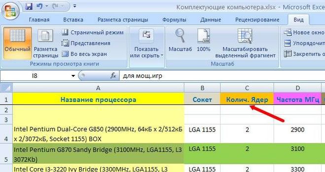 

Step 3

After we do not need to fix the cap, it can be removed. You need to open the “Freeze areas” item again, and there find the item “Unpin areas”. Accordingly, you need to make one left click on it.

After we have completed these steps, there will be no black line that separated the fixed line from the rest. If we try to scroll the table, we will see that the top line will very quickly go up off the screen. If we talk about older versions of Excel (2003 and older), then this operation is performed there in this way:

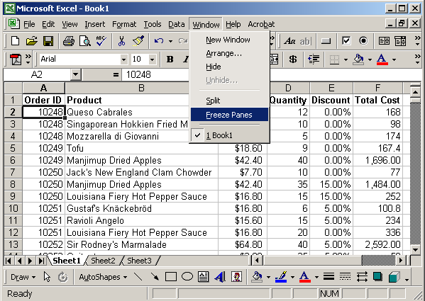
1. First, you need to select the first cell of the row immediately after the one we need to fix. In our case, this is cell A2.
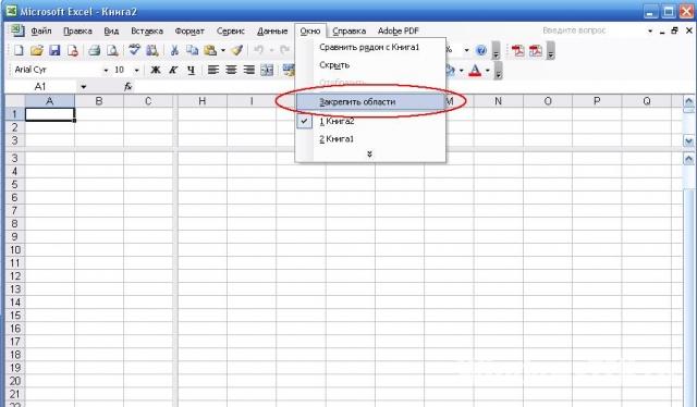
2. Next, click on the “Window” menu item and click on the “Freeze panes” button. 

If you need to pin several rows, then you just need to select the cell that immediately follows the last row that you want to pin. That is, if we need to select the first three lines, then we need to select cell A4, respectively.

If you want to freeze a region in Excel 2003, you must select the top cell of the next column. The logic is the same. If you need to freeze both a column and a row, then you need to find the cell that is the top left cell of the range that should be scrolled.

For example, if we need to freeze an area with two rows and two columns, then we need to select cell C3. After that, follow the same steps as described above.

As you can see, there is no fundamental difference. It’s just that the option is in a different menu. We also see that more modern versions of Excel make it possible to simply fix the first row without going into additional nuances. This is very convenient when you need to submit a report on time, and there is very little time left.

How to freeze a row in Excel on scroll

Since most often the table header is indicated in the first line, the sequence of actions in this case will be the same. But for clarity, let’s give another example that can demonstrate some additional nuances. Suppose we have such a table.

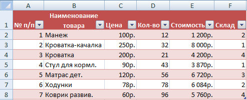
Usually there is only one heading in a table. Sometimes it contains one line, sometimes several. If the case is as we described in this picture, then the sequence of actions is as follows:

1. First, we create a table with these parameters.
2. Then we activate any cell of the table. If we are working with Excel version 2007, there is no fundamental difference for us which one to select, since there is a special function to fix the top row.
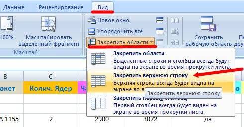
3. Expand the contents of the “View” tab. There we find the menu item “Freeze areas”. We click on it. After that, a list will appear in which you need to select the “Lock the top line” function. 

After that, we will see that a black line appears under our top line, which will separate the blocks of cells that scroll and the line, which will remain in one place until the user disables this feature.

Let’s assume a different situation. Let’s say a person needs to make several lines immovable when the sheet data is scrolled down. This should be done, for example, in order to check up-to-date data with the very first information. What can be done for this?

1. Click on any cell that is located under the line that needs to be fixed. So we tell the program which lines we should fix. 
2. After we do this, both the header row and the first row of the table itself will not move.

The principle with Excel version 2003 is similar.

How to freeze a column in Excel

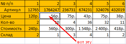
Suppose we have a horizontally oriented table, and therefore the names are fixed not in columns, but in rows. If you need to do this, the sequence of actions is as follows:

1. We make a click on any cell of the table. Which one is not so important, because Excel will automatically select the first column from the available data.
2. After that, go to the “Freeze Areas” menu described earlier, and there we find the item “Freeze first column”. 
3. Now, when we try to scroll the sheet to the left, the first column will stay in place.

To fix multiple columns, click on the lowest cell of the table column that follows the last column.

How to freeze row and column at the same time

Okay, let’s say we want to freeze an area that has two columns and two rows. To do this, we need to activate, as we know, the cell that is located at the intersection of rows and columns, but at the same time immediately behind the fixed area, and not inside it. It should be located simultaneously near the last fixed row, and near the last fixed column.

Next, click on the tool button “Lock areas”, and in the list of functions that appears, select the first item.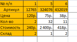 

How to unfreeze a row or column in Excel

Here’s another example that describes how to unfreeze a row or column. So, we need to click on the “Freeze area” button. Then a list of functions will appear in which we need, as we know, to click the “Unpin areas” button. After we click on this button, all areas that were previously fixed will be unpinned.

If you need to remove the fastening of a row in Excel 2003 version and older, then this button is located in the “Window” item. You can also add corresponding buttons to the toolbar. To do this, just right-click on the corresponding item and select the correct option.

Thus, we figured out how to fix the table header when scrolling, regardless of where exactly it is located: in rows or columns. And no matter what the weather is outside the window, you will know how to do it. Before performing in practice, it is recommended to practice so that in a situation where these skills are needed, do not get lost, but quickly press the necessary buttons. After all, the labor market loves highly effective employees, and every second counts.

In general, there is nothing complicated about freezing a row or column. It is enough just to press a few buttons that were described above. If you need to remove the pinning of lines, just one button is enough.