


Contents
When creating charts in Excel, the source data for it is not always on the same sheet. Fortunately, Microsoft Excel provides a way to plot data from two or more different worksheets in the same chart. See below for detailed instructions.
How to create a chart from data in multiple sheets in Excel
Let’s assume that there are several sheets with income data for different years in one spreadsheet file. Using this data, you need to build a chart to visualize the big picture.
1. We build a chart based on the data of the first sheet
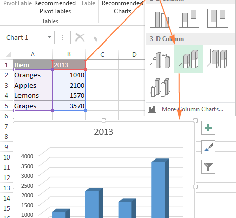
Select the data on the first sheet that you want to display in the chart. Further open the masonry Insert. In a group Diagrams Select the desired chart type. In our example, we use Volumetric Stacked Histogram.
It is the stacked bar chart that is the most popular type of charts used.
2. We enter data from the second sheet
Highlight the created diagram to activate the mini panel on the left Chart tools. Next, select Constructor and click on the icon Select data.
You can also click the button Chart Filters ![]() . On the right, at the very bottom of the list that appears, click Select data.
. On the right, at the very bottom of the list that appears, click Select data.
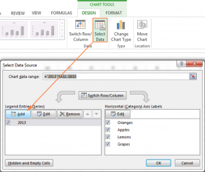
In the window that appears Source selection data follow the link Add.
We add data from the second sheet. This is an important point, so be careful.
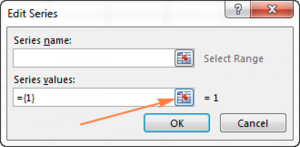
When you press a button Add, a dialog box pops up Row change. Near the field Value you need to select the range icon.
Window Row change curl up. But when switching to other sheets, it will remain on the screen, but will not be active. You need to select the second sheet from which you want to add data.
On the second sheet, it is necessary to highlight the data entered into the chart. To window Row changes activated, you just need to click on it once.
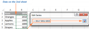
In order for a cell with text that will be the name of the new row, you need to select the data range next to the icon Row name. Minimize the range window to continue working in the tab Row changes.
Make sure the links in the lines Row name и The values indicated correctly. Click OK.
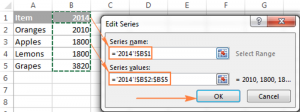
As you can see from the image attached above, the row name is associated with the cell V1where it is written. Instead, the title can be entered as text. For example, the second row of data.
The series titles will appear in the chart legend. Therefore, it is better to give them meaningful names.
At this stage of creating a diagram, the working window should look like this:
3. Add more layers if necessary
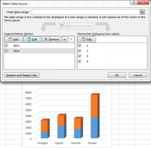
If you still need to insert data into the chart from other sheets Excel, then repeat all the steps from the second paragraph for all tabs. Then we press OK in the window that appears Selecting a data source.
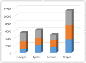
In the example there are 3 rows of data. After all the steps, the histogram looks like this:
4. Adjust and improve the histogram (optional)
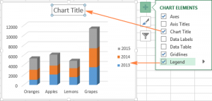
When working in Excel 2013 and 2016 versions, a title and a legend are automatically added when a bar chart is created. In our example, they were not added, so we will do it ourselves.
Select a chart. In the menu that appears Chart elements press the green cross and select all the elements that need to be added to the histogram:
Other settings, such as the display of data labels and the format of the axes, are described in a separate publication.
We make charts from the total data in the table
The charting method shown above only works if the data on all document tabs is in the same row or column. Otherwise, the diagram will be illegible.
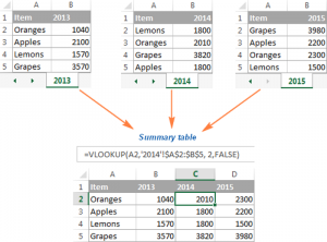
In our example, all data is located in the same tables on all 3 sheets. If you are not sure that the structure is the same in them, it would be better to first compile the final table, based on the available ones. This can be done using the function VLOOKUP or Merge Table Wizards.
If in our example all tables were different, then the formula would be:
=VLOOKUP (A3, ‘2014’!$A$2:$B$5, 2, FALSE)
This would result in:
After that, just select the resulting table. In the tab Insert find Diagrams and choose the type you want.
Editing a chart created from data on multiple sheets
It also happens that after plotting a graph, data changes are required. In this case, it is easier to edit an existing one than to create a new diagram. This is done through the menu. Working with charts, which is no different for graphs built from the data of one table. Setting the main elements of the graph is shown in a separate publication.
There are several ways to change the data displayed on the chart itself:
- through the menu Selecting a data source;
- via Filters
- I mediate Data series formulas.
To open the menu Selecting a data source, required in the tab Constructor press submenu Select data.
To edit a row:
- select a row;
- click on tab Change;
- change Value or First name, as we did before;
To change the order of rows of values, you need to select the row and move it using the special up or down arrows.
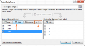
To delete a row, you just need to select it and click on the button Delete. To hide a row, you also need to select it and uncheck the box in the menu legend elements, which is on the left side of the window.
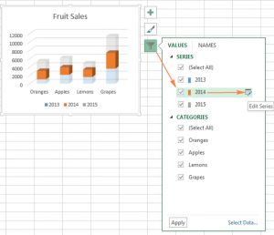
Modifying Series Through the Chart Filter
All settings can be opened by clicking on the filter button ![]() . It appears as soon as you click on the chart.
. It appears as soon as you click on the chart.
To hide data, just click on Filter and uncheck lines that should not be in the chart.
Hover the pointer over the row and a button appears Change row, click on it. A window pops up Selecting a data source. We make the necessary settings in it.
Note! When you hover the mouse over a row, it is highlighted for better understanding.
Editing a series using a formula
All series in a graph are defined by a formula. For example, if we select a series in our chart, it will look like this:
=SERIES(‘2013′!$B$1,’2013′!$A$2:$A$5,’2013’!$B$2:$B$5,1)
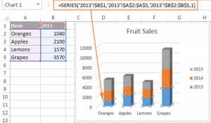
Any formula has 4 main components:
=SERIES([Series name], [x-values], [y-values], row number)
Our formula in the example has the following explanation:
- Series name (‘2013’!$B$1) taken from cell B1 on the sheet 2013.
- Rows value (‘2013’!$A$2:$A$5) taken from cells A2: A5 on the sheet 2013.
- Columns value (‘2013’!$B$2:$B$5) taken from cells B2: B5 on the sheet 2013.
- The number (1) means that the selected row has the first place in the chart.
To change a specific data series, select it in the chart, go to the formula bar and make the necessary changes. Of course, you must be very careful when editing a series formula, because this can lead to errors, especially if the original data is on a different sheet and you cannot see it when editing the formula. Still, if you’re an advanced Excel user, you might like this method, which allows you to quickly make small changes to your charts.