How to calculate percentages in Excel – with formula examples

This text provides detailed information about the interest calculation method in Excel, describes the main and additional formulas (increase or decrease the value by a specific percentage).

There is almost no area of ​​life in which the calculation of interest would not be required. It can be a tip for the waiter, a commission to the seller, income tax or mortgage interest. For example, were you offered a 25 percent discount on a new computer? To what extent is this offer beneficial? And how much money will you have to pay, if you subtract the amount of the discount.

Today you will be able to perform various percentage operations in Excel more efficiently.

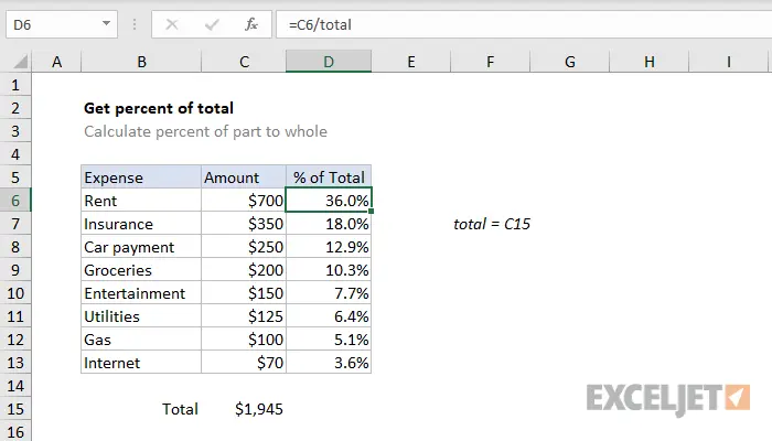
The basic formula for determining percentages of the total value

The word “percentage” is of Latin origin. This language has a construction “per centum”, which translates as “one hundred”. Many people from the lessons of mathematics can remember what formulas exist.

A percentage is a fraction of the number 100. To get it, you need to divide the number A by the number B and multiply the resulting number by 100.

Actually, the basic formula for determining percentages is as follows:

(Part number/Whole number)*100.

Let’s say you have 20 tangerines, and you want to give 5 of them for the New Year. How much is it in percentage? After performing simple operations (=5/20*100), we get 25%. This is the main method of calculating the percentage of a number in ordinary life.

In Excel, determining percentages is even easier because most of the work is done by the program in the background.

It is a pity, but there is no unique method that allows you to perform all existing types of operations. Everything is influenced by the required result, for the achievement of which the calculations are performed.

Therefore, here are some simple operations in Excel, such as determining, increasing / decreasing the amount of something in percentage terms, obtaining the quantitative equivalent of a percentage.

The main method for determining percentages in Excel

Part/Total = percentage

When comparing the main formula and the methodology for determining percentages in spreadsheets, you can see that in the latter situation there is no need to multiply the resulting value by 100. This is because Excel does this on its own if you first change the cell type to “percentage”.

And what are some practical examples of determining the percentage in Excel? Suppose you are a seller of fruits and other foodstuffs. You have a document that indicates the number of things ordered by customers. This list is given in column A, and the number of orders in column B. Some of them must be delivered, and this number is given in column C. Accordingly, column D will show the proportion of products delivered. To calculate it, you need to follow these steps:

1. Indicate =C2/B2 in cell D2 and move it down by copying it to the required number of cells.
2. Click on the “Percentage Format” button on the “Home” tab in the “Number” section.
3. Remember to increase the number of digits after the decimal point if necessary.

That’s all.

If you start using a different method of calculating interest, the sequence of steps will be the same.

In this case, the rounded percentage of products delivered is displayed in column D. To do this, remove all decimal places. The program will automatically display the rounded value.

It’s done this way

Determining a fraction of an integer value

The case of determining the share of an integer as a percentage described above is quite common. Let’s describe a number of situations where the acquired knowledge can be applied in practice.

Case 1: the integer is at the bottom of the table in a specific cell

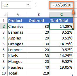
People often put an integer value at the end of a document in a specific cell (usually the bottom right). In this situation, the formula will take the same form as the one that was given earlier, but with a slight nuance, since the cell address in the denominator is absolute (that is, it contains a dollar, as shown in the picture below).

The dollar sign $ gives you the ability to bind a link to a specific cell. Therefore, it will remain the same, although the formula will be copied to a different location. So, if several readings are indicated in column B, and their total value is written in cell B10, it is important to determine the percentage using the formula: =B2/$B$10.

If you want the address of cell B2 to change depending on the location of the copy, you must use a relative address (without the dollar sign).

If the address is written in the cell $B$10, in which case the denominator will be the same up to row 9 of the table below.

Recommendation: To convert a relative address into an absolute address, you must enter a dollar sign in it. It is also possible to click on the required link in the formula bar and press the F4 button.

Here is a screenshot showing our result. Here we formatted the cell so that fractions up to a hundredth are displayed.

Example 2: parts of a whole are listed on different lines

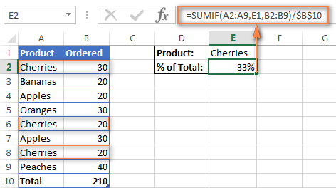
For example, let’s say we have a product that requires multiple stitches, and we need to understand how popular this product is against the backdrop of all the purchases made. Then you should use the SUMIF function, which makes it possible to first add all the numbers that can be attributed to a given heading, and then divide the numbers related to this product by the result obtained in the process of addition.

For simplicity, here is the formula:

=SUMIF(value range, condition, summation range)/sum.

Since column A contains all the product names, and column B indicates how many purchases were made, and cell E1 describes the name of the required product, and the sum of all orders is cell B10, the formula will look like this:

=SUMIF(A2:A9 ,E1, B2:B9) / $B$10.

Also, the user can prescribe the name of the product directly in the condition:

=SUMIF(A2:A9, «cherries», B2:B9) / $B$10.

If it is important to determine a part in a small set of products, the user can prescribe the sum of the results obtained from several SUMIF functions, and then indicate the total number of purchases in the denominator. For example, like this:

=(SUMIF(A2:A9, «cherries», B2:B9) + SUMIF(A2:A9, «apples», B2:B9)) / $B$10.

How to calculate the degree of correction of a value as a percentage in Excel

There are many calculation methods. But, probably, the formula for determining the change in percentage is used most often. To understand how much the indicator has increased or decreased, there is a formula:

Percent change = (BA) / A.

When doing actual calculations, it is important to understand which variable to use. For example, a month ago there were 80 peaches, and now there are 100. This indicates that you currently have 20 more peaches than before. The increase was 25 percent. If before that there were 100 peaches, and now there are only 80, then this indicates a decrease in the number by 20 percent (since 20 pieces out of a hundred is 20%).

Therefore, the formula in Excel will look like this: (New value – old value) / old value.

And now you need to figure out how to apply this formula in real life.

Example 1: calculating the change in value between columns

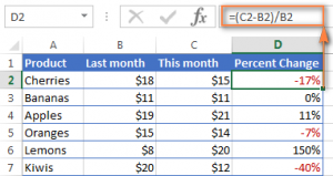
Let’s say that column B shows prices for the last reporting period, and column C shows prices for the current one. Then enter the following formula in cell C2 to find out the rate of change in value:

= (C2-B2) / B2

It measures the extent to which the value of the products listed in column A has increased or decreased compared to the previous month (column B).

After copying the cell to the remaining rows, set the percentage format so that numbers after zero are displayed appropriately. The result will be the same as in the screenshot.

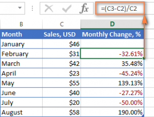
In this example, positive trends are shown in black and negative trends in red.

Example 2: calculating the rate of change between rows

If there is only a single column of numbers (for example, C containing daily and weekly sales), you will be able to calculate the percentage change in price using this formula:

= (S3-S2) / S2.

C2 is the first and C3 is the second cell.

Note. You should skip the 1st line and write the necessary formula in the second cell. In the given example, this is D3.

After applying the percentage format to the column, the following result will be produced.

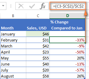
If it is important for you to find out the degree of value modification for a particular cell, you need to set up the link using absolute addresses containing the dollar sign $.

So, the formula for calculating the change in the number of orders in February compared to the first month of the year is as follows:

=(C3-$C$2)/$C$2.

When you copy a cell to other cells, the absolute address does not change as long as the relative one starts to refer to C4, C5, etc.

Calculation of interest in quantitative terms

As you have already seen, any calculations in Excel are quite an easy task. Knowing the percentage, it is easy to understand how much it will be from the whole in digital terms.

Example 1: calculating a share of the total

Let’s say you buy a laptop for $950 and you have to pay 11% tax on the purchase. How much money will have to be paid in the end? In other words, how much would 11% of $950 be?

The formula is:

Integer * percent = share.

If we assume that the whole is in cell A2, and the percentage is in cell B2, it is transformed into a simple = A2 * B2  The value $104,50 appears in the cell.

Remember that when you write a value displayed with a percent sign (%), Excel interprets it as a hundredth. For example, 11% is read by the program as 0.11, and Excel uses this figure in all calculations.

In other words, formula =A2*11% analogous =A2*0,11. Naturally, you can use the value 0,11 instead of a percentage directly in the formula if that’s more convenient at the time.

Example 2: finding the whole from a fraction and a percentage

For example, a friend offered you his old computer for $400, which is 30% of its purchase price, and you need to know how much a new computer costs.

First you need to determine how many percent of the original price a used laptop costs.

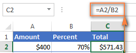
It turns out that its price is 70 percent. Now you need to know the formula for calculating the original cost. That is, to understand from what number 70% will be 400. The formula is as follows:

Share of the total / percentage = total value.

If applied to real data, it could take one of the following forms: =A2/B2 or =A2/0.7 or =A2/70%.

How to change a number to some percentage

Suppose the holiday season has begun. Naturally, everyday spending will be affected, and you may want to consider alternative possibilities to find the optimal weekly amount by which weekly spending can increase. Then it is useful to increase the number by a certain percentage.

To increase the amount of money by interest, you need to apply the formula:

= value * (1+%).

For example, in the formula =A1*(1+20%) the value of cell A1 is increased by a fifth.

To decrease the number, apply the formula:

= Meaning * (1–%).

Yes, the formula = A1*(1-20%) reduces the value in cell A1 by 20%.

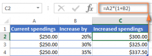
In the example described, if A2 is your current costs and B2 is the percentage you should change them by, you need to write formulas in cell C2:

1. Percent increase:  =A2*(1+B2).
2. Decrease by percentage: =A2*(1-B2).

How to increase or decrease all values ​​of an entire column by a percentage

How to change all values ​​in a column to a percentage?

Let’s imagine that you have a column of values ​​that you need to change to some part, and you want to have the updated values ​​in the same place without adding a new column with a formula. Here are 5 easy steps to complete this task:

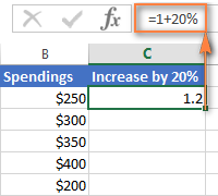
1. Enter all values ​​that require correction in a specific column. For example, in column B.
2. In an empty cell, write one of the following formulas (depending on the task):
   1. Increase: =1+20%
   2. Decrease: =1-20%.

Naturally, instead of “20%” you need to specify the required value.

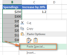
1. Select the cell in which the formula is written (this is C2 in the example we are describing) and copy by pressing the key combination Ctrl + C.
2. Select a set of cells that need to be changed, right-click on them and select “Paste Special …” in the English version of Excel or “Paste Special” in .

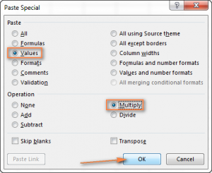
1. Next, a dialog box will appear in which you need to select the “Values” parameter (values), and set the operation as “Multiply” (multiply). Next, click on the “OK” button.

And here is the result – all the values ​​in column B have been increased by 20%.

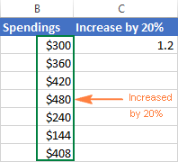
Among other things, you can multiply or divide columns with values ​​by a certain percentage. Just enter the desired percentage in the empty box and follow the steps above.