Comparing 2 files in Excel for differences

Each user may encounter a situation where they need to compare two tables. Well, as a last resort, everyone has to compare two columns. Yes, of course, working with Excel files is highly convenient and comfortable. Sorry, this is not a comparison. Of course, visual sorting of a small table is possible, but when the number of cells goes into the thousands, you have to use additional analytical tools.

Unfortunately, a magic wand has not yet been opened that allows you to automatically compare all the information with each other in one click. Therefore, you have to work, namely, to collect data, specify the necessary formulas and perform other actions that allow you to automate comparisons at least a little.

There are many such actions. Let’s look at some of them.

What is the purpose of comparing Excel files?

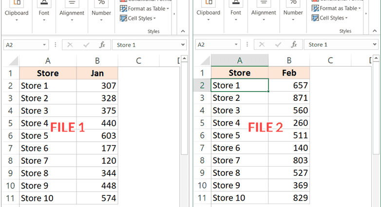
There can be a huge number of reasons why several Excel files are compared. Sooner or later, each user is faced with such a need, and he does not have such questions. For example, you might want to compare data from two reports for different quarters to see if financials have gone up or down.

Or, alternatively, the teacher needs to see which students were kicked out of the university by comparing the composition of the student group last year and this year.

There can be a huge number of such situations. But let’s move on to practice, because the topic is quite complex.

All Ways to Compare 2 Tables in Excel

Although the topic is complex, it is easy. Yes, don’t be surprised. It is complex because it is made up of many parts. But these parts themselves are easy to understand and perform. Let’s look at how you can compare two Excel spreadsheets, directly in practice.

Equality Formula and False-True Test

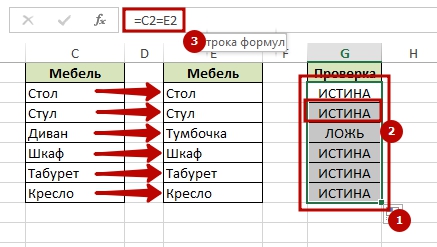
Let’s start, of course, with the simplest method. This method of comparing documents is possible, and within a fairly wide range. You can compare not only text values, but also numeric ones. And let’s take a little example. Let’s say we have two ranges with number format cells. To do this, simply write the equality formula =C2=E2. If it turns out that they are equal, “TRUE” will be written in the cell. If they differ, then FALSE. After that, you need to transfer this formula to the entire range using the autocomplete marker.

Now the difference is visible to the naked eye.

Highlighting Distinct Values

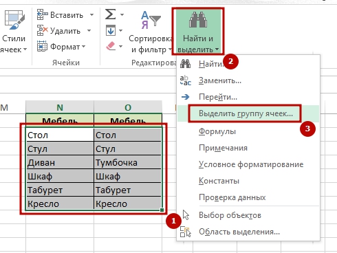
You can also make values ​​that differ from each other highlighted in a special color. This is also a pretty simple task. If it is enough for you to find differences between two ranges of values ​​or entire tables, you need to go to the “Home” tab, and select the “Find and highlight” item there. Before you click it, be sure to highlight the set of cells that store information for comparison. 

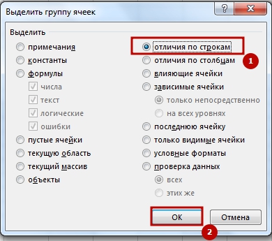
In the menu that appears, click on the menu “Select a group of cells …”. Next, a window will open in which we need to select differences by lines as a criterion.

Comparing 2 tables using conditional formatting

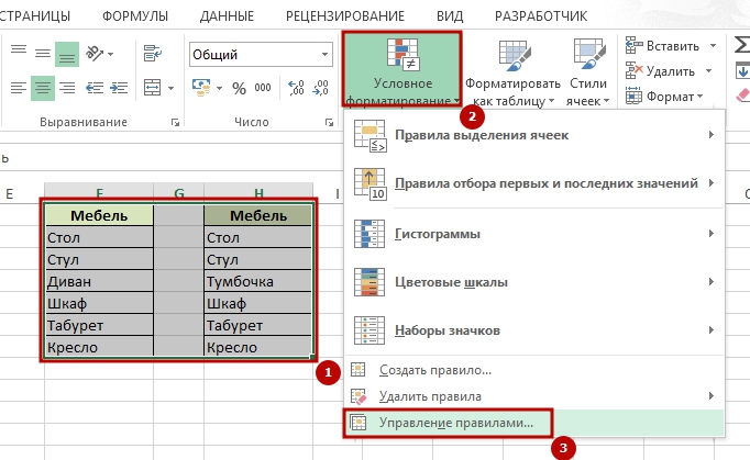
Conditional formatting is a very convenient and, importantly, functional method that allows you to choose a color that will highlight a different or the same value. You can find this option on the Home tab. There you can find a button with the appropriate name and in the list that appears, select “Manage rules”. A rule manager will appear, in which we need to select the “Create Rule” menu.

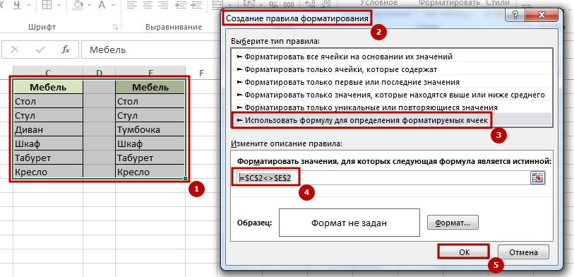
Next, from the list of criteria, we need to select the one where it says that we need to use a formula to determine the cells that will be formatted in a special way. In the description of the rule, you need to specify a formula. In our case, this is =$C2<>$E2, after which we confirm our actions by pressing the “Format” button. After that, we set the appearance of the cell and see if we like it through a special mini-window with a sample. 

If everything suits, click the “OK” button and confirm the actions.

In the Conditional Formatting Rules Manager, the user can find all the formatting rules that are in effect in this document. 

COUNTIF function + table comparison rules

All the methods that we described earlier are convenient for those formats whose format is the same. If the tables were not previously ordered, then the best method is to compare two tables using the function COUNTIF and rules. 

Let’s imagine that we have two ranges with slightly different information. We are faced with the task of comparing them and understanding which value is different. First you need to select it in the first range and go to the “Home” tab. There we find the previously familiar item “Conditional Formatting”. We create a rule and set the rule to use a formula. 

In this example, the formula is as shown in this screenshot.

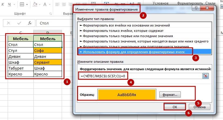
After that, we set the format as described above. This function parses the value contained in cell C1 and looks at the range specified in the formula. It corresponds to the second column. We need to take this rule and copy it over the entire range. Hooray, all cells with non-repeating values ​​are highlighted.

VLOOKUP function to compare 2 tables

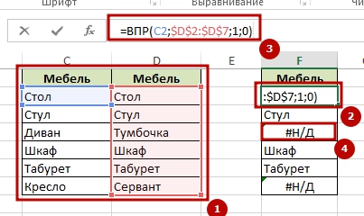
In this method, we will consider the function VPR, which checks if there are any matches in two tables. To do this, you need to enter the formula shown in the picture below and transfer it to the entire range that is used for comparison.

This function iterates over each value and sees if there are any duplicates from the first column to the second. Well, after performing all the operations, this value is written in the cell. If it is not there, then we get the #N/A error, which is quite enough to automatically understand which value will not match.

IF function

Logic function IF – this is another good way to compare two ranges. The main feature of this method is that you can use only the part of the array that is being compared, and not the entire table. This saves resources for both the computer and the user.

Let’s take a small example. We have two columns – A and B. We need to compare some of the information in them with each other. To do this, we need to prepare another service column C, in which the following formula is written.

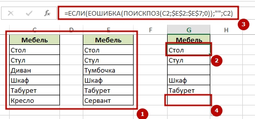
Using a formula that uses functions IF, IFERROR и MORE EXPOSED you can iterate over all the desired elements of column A, and then in column B. If it was found in columns B and A, then it is returned to the corresponding cell.

VBA macro

A macro is the most complex, but also the most advanced method of comparing two tables. some comparison options are generally not possible without VBA scripts. They allow you to automate the process and save time. All the necessary operations for data preparation, if programmed once, will continue to be performed.

Based on the problem to be solved, you can write any program that compares data without any user intervention.

How to compare files in Excel

If the user has set himself the task (well, or he has been given one) to compare two files, then this can be done by two methods at once. The first one is using a specialized function. To implement this method, follow the instructions:

1. Open the files you want to compare.
2. Open the tab “View” – “Window” – “View side by side”.

After that, two files will be opened in one Excel document.

The same can be done with commonplace Windows tools. First you need to open two files in different windows. After that, take one window and drag it to the very left side of the screen. After that, open a second window and drag it to the very right side. After that, the two windows will be side by side. 

Conditional formatting to compare 2 excel files

Very often comparing documents means displaying them next to each other. But in some cases, it is possible to automate this process using conditional formatting. With it, you can check if there are differences between the sheets. This allows you to save time that can be used for other purposes.

First, we need to transfer the compared sheets into one document. 

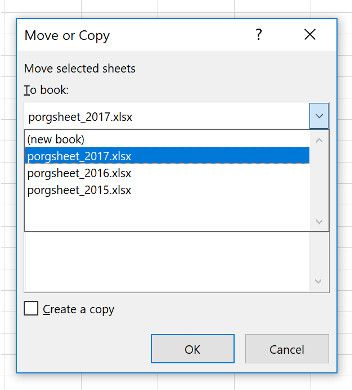
To do this, you need to right-click on the appropriate sheet, and then click on the “Move or copy” button in the pop-up menu. Next, a dialog box will appear in which the user can select the document in which this sheet should be inserted.

Next, you need to select all the desired cells to display all the differences. The easiest way to do this is by clicking the top left cell, and then pressing the key combination Ctrl + Shift + End.

After that, go to the conditional formatting window and create a new rule. As a criterion, we use a formula suitable in a particular case, then we set the format.

Attention: the addresses of the cells must be indicated those that are on another sheet. This can be done through the formula input menu.

Comparing data in Excel on different sheets

Suppose we have a list of employees that also lists their salaries. This list is updated every month. This list is copied to a new sheet.

Suppose we need to compare salaries. In this case, you can use tables from different sheets as data. We will use conditional formatting to highlight the differences. Everything is simple.

With conditional formatting, you can make effective comparisons even if the names of the employees are in a different order.

How to compare 2 sheets in excel spreadsheet

Comparison of information located on two sheets is carried out using the function MORE EXPOSED. As its first parameter, there is a pair of values ​​that you need to look for on the sheet that is responsible for the next month. Simply put, March. We can designate the viewed range as a collection of cells that are part of the named ranges, combined in pairs.

So you can compare strings according to two criteria – last name and salary. Well, or any other, defined by the user. For all matches that could be found, a number is written in the cell in which the formula is entered. For Excel, this value will always be true. Therefore, in order for the formatting to be applied to those cells that were different, you need to replace this value with LYING, using the function =NOT().

Spreadsheet Compare Tool

Excel has a special tool that allows you to compare spreadsheets and highlight changes automatically. 

It is important to note that this tool is available only to those users who have purchased Professional Plus office suites.

You can open it directly from the “Home” tab by selecting the “Compare Files” item.

After that, a dialog box will appear in which you need to select the second version of the book. You can also enter the Internet address where this book is located.

After we select two versions of the document, we need to confirm our actions with the OK key.

In some cases, an error may be generated. If it appears, it may indicate that the file is password protected. After you click OK, you will be prompted to enter it. 

The comparison tool looks like two Excel spreadsheets next to each other within the same window. Depending on whether information has been added, removed, or there has been a change in the formula (as well as other types of actions), the changes are highlighted in different colors. 

How to interpret comparison results

It’s very simple: different types of differences are indicated by different colors. Formatting can extend to both the cell fill and the text itself. So, if data was entered into the cell, then the fill is green. If something becomes unclear, the service itself has symbols that show what type of change is highlighted in what color.