CONCATENATE function in Excel – usage guide with examples

From time to time it may be necessary to combine the values ​​contained in different cells into one. The & symbol is usually used for this. But its functionality is somewhat limited as it cannot concatenate multiple strings.

This simple function is replaced by a more functional version of it – STsEPIT. In fact, in modern versions of Microsoft Office, this function is no longer there, it is completely replaced by the function STEP. It’s still usable for now, it’s included for backwards compatibility, but after a while it might not be. Therefore, it is recommended that in Excel 2016, Online and newer versions, use the function STEP.

CONCATENATE function – detailed description

Function STsEPIT refers to text. This means that it is used to perform operations on text values. At the same time, you can specify arguments in different formats: text, numeric, or as cell references. 

In general, the rules for using this feature are as follows:

1. A semicolon is used to separate arguments. If the user decides to use other characters, then the display will be the result in quotation marks.
2. If a value in text format is used as a function argument and is entered directly into a formula, it must be enclosed in quotation marks. If there is a reference to such a value, then no quotes are required. The same goes for numeric values. If you need to add a digit to a string, then the quote is not required. If you violate these rules, the following error will be displayed – #NAME?
3. If you need to add a space between the connected elements, it must be added as a separate text string, that is, in quotation marks. Like this: ” ” .

Now let’s take a closer look at the syntax of this function. He is very simple. 

Syntax

So, in fact, there is only one argument – this is a text string that should be inserted. Each argument, as we already know, is separated by a semicolon. You can specify up to 255 arguments. They themselves are duplicated in their own way. The first argument is required. And as we already know, you can specify arguments in three formats: text, number, and link. 

Applications of the CONCATENATE function

Number of application areas of the function STsEPIT huge. In fact, it can be applied almost everywhere. Let’s look at some of them in more detail:

1. Accounting. For example, an accountant is tasked with highlighting the series and document number, and then inserting this data as one line in one cell. Or you need to add to the series and number of the document by whom it was issued. Or list several receipts in one cell at once. In fact, there are a whole bunch of options, you can list indefinitely. 
2. Office reports. Especially if you need to provide summary data. Or combine first and last name.
3. Gamification. This is a very popular trend that is actively used in education, parenting, as well as in loyalty programs of various companies. Therefore, in the field of education and business, this function can also be useful. 

This function is included in the standard set that every Excel user should know. 

Inverse CONCATENATE function in Excel

In fact, there is no such function that would be completely opposite to the “CONCATENATE” function. To perform cell splitting, other functions are used, such as LEVSIMV и RIGHTand PSTR. The first extracts a certain number of characters from the left of the string. The second one is on the right. BUT PSTR can do it from an arbitrary place and end in an arbitrary place. 

You may also need to perform more complex tasks, but there are separate formulas for them. 

Common problems with the CONCATENATE function

At first glance, the function STsEPIT pretty simple. But in practice, it turns out that a whole bunch of problems are possible. Let’s take a closer look at them. 

1. Quotes are displayed in the result string. To avoid this problem, you need to use a semicolon as a separator. But, as mentioned above, this rule does not apply to numbers.
2. The words are very close. This problem occurs because a person does not know all the nuances of using the function STsEPIT. To display words separately, you must add a space character to them. Or you can insert it directly after the text argument (both inside the cell and if you enter the text separately in the formula). For example like this: =CONCATENATE(“Hello”, “dear”). We see that here a space has been added to the end of the word “Hello”. 
3. #NAME? This indicates that no quotes were specified for the text argument. 

Recommendations for using the function

To make working with this function more efficient, you need to consider several important recommendations:

1. Use & as much as possible. If you need to join just two text lines, then there is no need to use a separate function for this. So the spreadsheet will run faster, especially on weak computers with a small amount of RAM. An example is the following formula: =A1 & B1. It is similar to the formula =SECTION(A1,B1). Especially the first option is easier when manually entering the formula.
2. If it is necessary to combine a currency or a date with a text string, as well as information in any other format other than those listed above, then you must first process it with the function TEXT. It is designed to convert numbers, dates, symbols into text.

As you can see, it is not difficult to understand these nuances at all. And they follow from the information above. 

Common Uses for the CONCATENATE Function

So the general formula is: CONCATENATE([text2];[text2];…). Insert your text in the appropriate places. It is important to note that the requirement for the received text is as follows: it must be less than the length of the field in which the value is entered. As attributes, you can use not only predefined values, but also information in cells, as well as the results of calculations using other formulas.

In this plan, there is no mandatory recommendation to use data for input in text format. But the final result will be displayed in the “Text” format.

There are several ways to enter a function: one manual and several semi-automatic. If you are a beginner, then it is recommended that you use the dialog box method of entering arguments. More experienced users of the program can also enter formulas manually. At first it will seem inconvenient, but in fact, nothing more efficient than keyboard input has yet been invented. 

By the way, the recommendation for using Excel in general: always learn hotkeys. They will help you save a lot of time.

But while you are a beginner, you will have to use a specially created window.

So how to call it? If you look at the formula input line, then to the left of it there is such a small button “fx”. If you press it, the following menu appears. We need to select the desired function from the list.

After we select the desired function, a window for entering arguments will open. Through it, you can set a range or manually enter text, a link to a cell. 

If you enter data manually, then the input is carried out, starting with an “equal” sign. That is, like this:

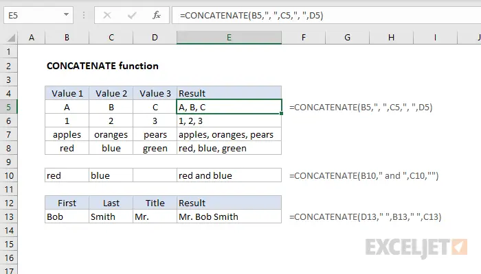
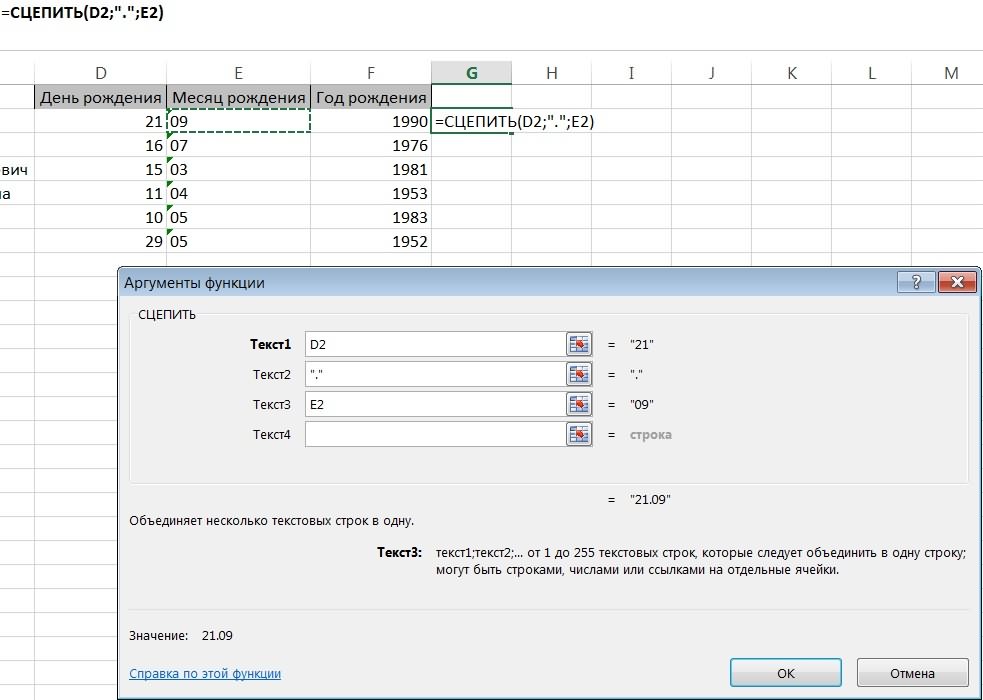
=CONCATENATE(D2;”,”;E2)

After all the operations performed by us, we will see in the resulting cell the text “21.09”, which consists of several parts: the number 21, which can be found in the cell indexed as D2 and line 09, which is in cell E2. In order for them to be separated by a dot, we used it as the second argument. 

Name binding

For clarity, let’s look at an example that describes how to bind names. 

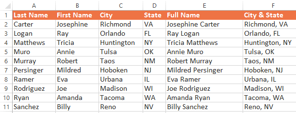
Let’s say we have such a table. It contains information about first name, last name, city, state of customers. Our task is to combine the first and last name and get the full name. 

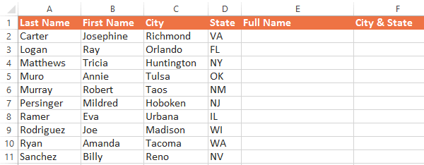
Based on this table, we understand that references to names should be given in column B, and last names – A. The formula itself will be written in the first cell under the heading “Full Name”.

Before entering a formula, remember that the function will not associate more information than the user has specified. Therefore, if you need to add delimiters, question marks, dots, dashes, spaces, they must be entered as separate arguments.

In our example, we need to separate the first and last name with a space. Therefore, we need to enter three arguments: the address of the cell containing the first name, a space character (do not forget to include it in quotation marks), and the address of the cell containing the last name. 

After we have defined the arguments, we write them into the formula in the appropriate sequence. 

It is very important to pay attention to the syntax of the formula. We always start it with an equal sign, after which we open the brackets, list the arguments, separating them with a semicolon, and then close the brackets.

Sometimes you can put a regular comma between the arguments. If the English version of Excel is used, then a comma is put. If the -language version, then a semicolon. After we press Enter, the merged version will appear.

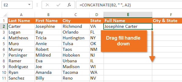
Now all that’s left is to simply use the autofill marker to insert this formula into all the other cells in this column. As a result, we have the full name of each client. Mission accomplished.

In exactly the same way, you can connect the state and the city.

Linking numbers and text

As we already know, using the function STsEPIT we can concatenate numeric values ​​with text values. Let’s say we have a table with data about the inventory of goods in a store. At the moment we have 25 apples, but this row is spread over two cells. 

We need the following end result.

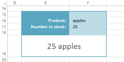
In this case, we also need three arguments, and the syntax is still the same. But let’s try to complete the task of a slightly increased complexity. Suppose we need to write the complex string “We have 25 apples”. Therefore, we need to add one more line “We have” to the three existing arguments. The end result looks like this.

=CONCATENATE(“We have “;F17;” “;F16)

If desired, the user can add almost as many arguments as he wants (within the above limit).

Connecting VLOOKUP and CONCATENATE

If you use functions VPR и STsEPIT together, it can turn out to be a very interesting and, importantly, functional combination. Using the function VPR we perform a vertical search on the table according to a certain criterion. Then we can add the found information to the already existing line.

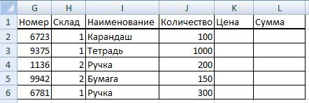
So, let’s say we have such a table. It describes what goods are currently in the first and second warehouses. 

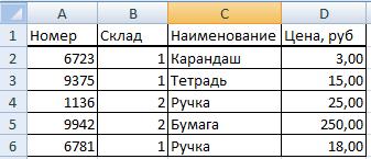
We need to find the price of a certain item in a certain warehouse. For this, the function is used VPR. But before using it, you must first prepare the table a little. VPR outputs data to the left, so you need to insert an additional column on the left of the table with the original data. 

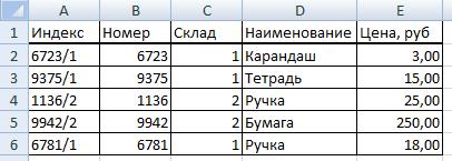
After that we concatenate the data. 

This can be done either with this formula:

=B2&»/»&C2

Or such.

=CONCATENATE(B2;”/”;C2)

Thus, we concatenated two columns together, using a forward slash as the separator between the two values. Next, we transferred this formula to the entire column A. We get such a table.

Next, we take the following table and fill it with information about the product selected by the visitor. We need to get information about the cost of the goods and the warehouse number from the first table. This is done using the function VPR.

Next, select a cell K2, and write the following formula in it. 

{=ВПР(G2&»/»&H2;A2:E6;5;0)}

Or it can be written through the function STsEPIT.

{=ВПР(СЦЕПИТЬ(G2;»/»;H2);A2:E6;5;ЛОЖЬ)}

The syntax in this case is similar to how the combination of information about the number and warehouse was carried out. 

You need to include a function VPR through the key combination “Ctrl” + “Shift” + “Enter”.

As you can see, everything is simple.