


After collecting, systematizing and processing data, it is often necessary to demonstrate them. Tables are great at presenting data row by row, but a chart can breathe life into it. A diagram creates a visual impact that conveys not only the data, but also their relationship and meaning.
The pie chart is an industry standard for conveying the relationship between parts and wholes. Pie charts are used when it is necessary to show how specific pieces of data (or sectors) contribute to the big picture. Pie charts are not suitable for showing data that changes over time. Also, don’t use a pie chart to compare data that doesn’t add up to a grand total at the end.
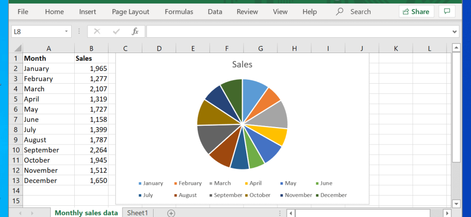
The following shows how to add a pie chart to an Excel sheet. The suggested methods work in Excel 2007-2013. Images are from Excel 2013 for Windows 7. Depending on the version of Excel you are using, individual steps may vary slightly.
Inserting a chart
In this example, we want to show the relationship between the different levels of donors who participate in a charity, compared to the total number of donations. The pie chart is perfect to illustrate this. Let’s start by summarizing the results for each level of donation.
- Select the range or table of data you want to show in the chart. Note that if the table has a row The overall result (Grand total), then this line does not need to be selected, otherwise it will be shown as one of the sectors of the pie chart.
- On the Advanced tab Insert (Insert) in section Diagrams (Charts) click on the pie chart icon. There are several standard charts to choose from. When hovering over any of the suggested chart options, a preview will be enabled. Choose the most suitable option.
Prompt! In Excel 2013 or newer versions, you can use the section Diagrams (Charts) tool Fast analysis (Quick Analysis), the button of which appears next to the selected data. In addition, you can use the button Recommended charts (Recommended Charts) tab Insert (Insert) to open the dialog Insert a chart (Insert charts).
★ Read more in the article: → How to make a pie chart in Excel, formulas, example, step by step instructions
Editing a Pie Chart
When the diagram is inserted in the right place, there will be a need to add, change or customize its various elements. Click on the chart you want to edit to bring up the tab group on the Ribbon Working with charts (Chart tools) and edit buttons. In Excel 2013, many options can be customized using the edit buttons next to the chart.
On the Design tab
- Add data labels, customize the chart title and legend. Click More options (More Options) to open the formatting panel and access even more options.
- Try to change Chart Style (Chart Style) and Chart colors (Chart Colors).
On the Format tab
- Edit and customize the style of the text in the title, legend, and more.
- Drag individual chart elements to new positions.
- Spread the sectors apart:
- To zoom out one sector, simply select it and drag it away from the chart.
- To remove all sectors from the center, right-click on the diagram and select Data series format (Format Data Series). On the panel that appears, click Sliced Pie Chart (Pie Explosion) to change the distance between the pieces.
- For a three-dimensional chart, you can adjust the thickness, rotation angle, add a shadow and other parameters of the chart itself and the plotting area.
The result is not only an informative illustration of the contribution of each group of donors to the cause of the organization, but also a beautifully designed graphic that is suitable for brochures, posters and placement on websites, respecting the corporate colors and style of your organization.