


Those who work in sales, marketing, or any other field that uses or receives reports from business software are probably familiar with the sales funnel. Try to create your own funnel chart and you will see that it takes some skill. Excel provides tools for creating inverted pyramids, but it takes some effort.
The following shows how to create a funnel chart in Excel 2007-2010 and Excel 2013.
How to Create a Funnel Chart in Excel 2007-2010
The images in this section were taken from Excel 2010 for Windows.
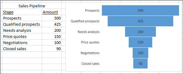
- Highlight the data you want to include in the chart. For example, let’s take the number of subscribers connected to the pipeline (column Number of Accounts in the Pipeline in the table below).
- On the Advanced tab Insert (Insert) click the button bar chart (Column) select Normalized stacked pyramid (100% stacked pyramid).
- Select a data series by clicking on any data point.
- On the Advanced tab Constructor (Design) in a group Data (Data) click the button Row column (Switch Row/Column).
- Right click on the pyramid and select XNUMXD Rotation (3-D Rotation) in the menu that appears.
- Change the angle of rotation along the axes X и Y at 0 °.
- Right-click on the vertical axis and from the menu that appears select Axis Format (Format Axis).
- Tick Reverse order of values (Values in reverse order) – the funnel chart is ready!
★ Read more in the article: → How to build a sales funnel chart in Excel
How to Create a Funnel Chart in Excel 2013
The images in this section were taken from Excel 2013 for Windows7.
- Highlight the data you want to include in the chart.
- On the Advanced tab Insert (Insert) select Volumetric stacked histogram (3-D Stacked Column chart).
- Right-click on any column and from the menu that appears select Data series format (Format Data Series). The panel of the same name will open.
- From the proposed form options, select complete pyramid (Full Pyramid).
- Select a data series by clicking on any data point.
- On the Advanced tab Constructor (Design) in the section Data (Data) click the button Row column (Switch Row/Column).
- Right-click on the pyramid and from the menu that appears select XNUMXD Rotation (3-D Rotation).
- In the panel that appears Chart Area Format (Format Chart Area) section XNUMXD Rotation (3-D Rotation) change the angle of rotation along the axes X и Y at 0 °.
- Right-click on the vertical axis and from the menu that appears select Axis Format (Format Axis).
- Tick Reverse order of values (Values in reverse order) – the funnel chart is ready!
Once your funnel chart is ready and facing the way you want, you can remove the data labels and chart title, and customize the design to your liking.
Prompt! If your chart isn’t based on a specific data series, or if you only want to convey an idea and not specific numbers, it’s easier to use a pyramid from the SmartArt graphic set.