Charts in Excel

A simple chart in Excel can say much more than a whole sheet filled with numbers. Creating charts in Excel is very easy – you will see for yourself.

Create a chart

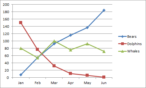
To create a line chart, follow these steps:

1. Highlight a range A1:D7.
2. On the Advanced tab Insert (Insert) in section Diagrams (Charts) click Insert Graph (Line) and select Graph with markers (Line with Markers).

Result:

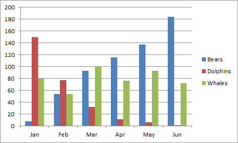
Changing the chart type

The initially selected chart type can be easily changed at any stage of work. For this:

1. Select a chart.
2. On the Advanced tab Insert (Insert) in section Diagrams (Charts) click Insert histogram (Column) and select Histogram with grouping (Clustered Column).

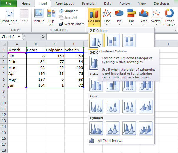
Result:

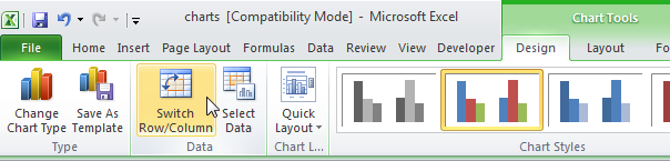
Swap rows and columns

To move the animal names displayed originally along the vertical axis to the horizontal axis, do the following:

1. Select a chart. A group of tabs will appear on the Menu Ribbon Working with charts (Chart Tools).
2. On the Advanced tab Constructor (Design) click Row column (Switch Row/Column).

Result:

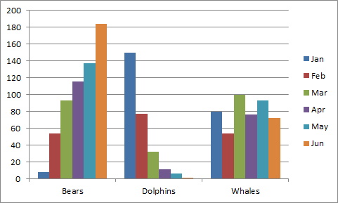
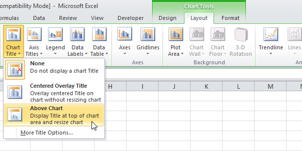
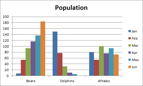
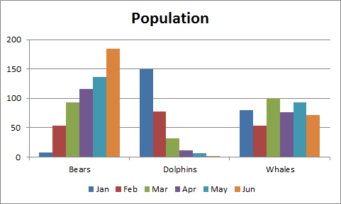
Chart title

To add a title to a chart, follow these steps:

1. Select a chart. A group of tabs will appear on the Menu Ribbon Working with charts (Chart Tools).
2. On the Advanced tab Layout (Layout) click Chart title (Chart Title) > Above chart (Above Chart).
3. Enter the title. In our example, we named the chart Population.

Result:

Legend position

By default, the legend is placed on the right side of the chart.

1. Select a chart. A group of tabs will appear on the Menu Ribbon Working with charts (Chart Tools).
2. On the Advanced tab Layout (Layout) click Legend (Legend) > Bottom (Show Legend at Bottom).

Result:

Data Signatures

Use data labels to focus readers on a particular data set or data point.

1. Select a chart. A group of tabs will appear on the Menu Ribbon Working with charts (Chart Tools).
2. Click on the orange column of the chart to highlight the data series Jun. Click again on the orange column to highlight one data point.
3. On the Advanced tab Layout (Layout) click Data Signatures (Data Labels) > At the edge, outside (Outside End).

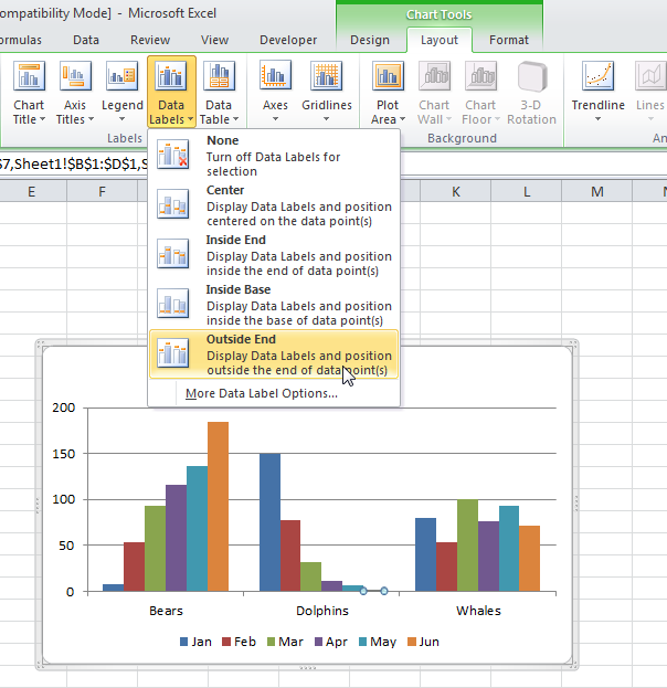
Result: