


From this guide you will learn and be able to learn how to hide columns in Excel 2010-2013. You will see how the standard Excel functionality for hiding columns works, and you will also learn how to group and ungroup columns using the “Grouping».
Being able to hide columns in Excel is very useful. There can be many reasons not to display some part of the table (sheet) on the screen:
- Two or more columns need to be compared, but they are separated by several other columns. For example, you would like to compare columns A и Y, and for this it is more convenient to place them side by side. By the way, in addition to this topic, you may be interested in the article How to Freeze Regions in Excel.
- There are several auxiliary columns with intermediate calculations or formulas that can confuse other users.
- You would like to hide from prying eyes or protect from editing some important formulas or personal information.
Read on to learn how Excel makes it quick and easy to hide unwanted columns. In addition, in this article you will learn an interesting way to hide columns using the “Grouping“, which allows you to hide and show hidden columns in one step.
Hide selected columns in Excel
Do you want to hide one or more columns in a table? Is there an easy way to do this:
- Open an Excel sheet and select the columns you want to hide.
Tip: To select non-adjacent columns, mark them by clicking the left mouse button while holding down the key Ctrl.
- Right-click on one of the selected columns to bring up the context menu and select Hide (Hide) from the list of available actions.
Tip: For those who love keyboard shortcuts. You can hide selected columns by clicking Ctrl + 0.
Tip: You can find a team Hide (Hide) on the Menu Ribbon Home > Cells > Framework > Hide and show (Home > Cells > Format > Hide & UnHide).
Voila! Now you can easily leave only the necessary data for viewing, and hide the not necessary so that they do not distract from the current task.
Use the “Group” tool to hide or show columns in one click
Those who work a lot with tables often use the ability to hide and show columns. There is another tool that does a great job with this task – you will appreciate it! This tool isGrouping“. It happens that on one sheet there are several non-contiguous groups of columns that need to be hidden or displayed sometimes – and do it again and again. In such a situation, grouping greatly simplifies the task.
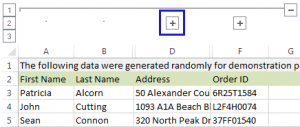
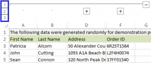
When you group columns, a horizontal bar appears above them to show which columns are selected for grouping and can be hidden. Next to the dash, you will see small icons that allow you to hide and show hidden data in just one click. Seeing such icons on the sheet, you will immediately understand where the hidden columns are and which columns can be hidden. How it’s done:
- Open an Excel sheet.
- Select the cells to hide.
- Press Shift+Alt+Right Arrow.
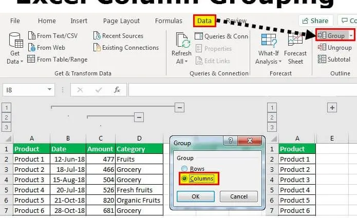
- A dialog box will appear Grouping (Group). Select Колонны (Columns) and click OKto confirm the selection.

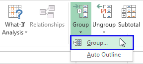
Tip: Another path to the same dialog box: Data > Group > Group (Data > Group > Group).
Tip: To ungroup, select the range containing the grouped columns and click Shift+Alt+Left Arrow.
- Tool «Grouping» will add special structure characters to the Excel sheet, which will show exactly which columns are included in the group.
- Now, one by one, select the columns you want to hide, and for each press Shift+Alt+Right Arrow.
Note: You can only group adjacent columns. If you want to hide nonadjacent columns, you will have to create separate groups.
- As soon as you press the key combination Shift+Alt+Right Arrow, hidden columns will be shown, and a special icon with the sign “—» (minus).
- Clicking on minus will hide the columns, and “—‘ will turn into ‘+“. Clicking on plus will instantly display all columns hidden in this group.
- After grouping, small numbers appear in the upper left corner. They can be used to hide and show all groups of the same level at the same time. For example, in the table below, clicking on a number 1 will hide all the columns that are visible in this figure, and clicking on the number 2 will hide the columns С и Е. This is very handy when you create a hierarchy and multiple levels of grouping.
That’s all! You have learned how to use the tool to hide columns in Excel. In addition, you learned how to group and ungroup columns. We hope that knowing these tricks will help you make your usual work in Excel much easier.
Be successful with Excel!