How to calculate markup percentage in Excel

In Microsoft Office Excel, it is possible to calculate the percentage of markup for a particular product in the shortest possible time by using a special formula. The details of the calculation will be presented in this article.

What is markup

In order to calculate this parameter, you must first understand what it is. Markup is the difference between the wholesale and retail cost of goods, leading to an increase in the price of products for the final consumer. The size of the margin depends on many factors, and it should cover the costs.

Pay attention! Margin and markup are two different concepts and should not be confused with each other. The margin is the net profit from the sale of goods, which is obtained after deducting the necessary costs.

How to Calculate Markup Percentage in Excel

There is no need to count manually. This is inappropriate, because. Excel allows you to automate almost any mathematical action, saving the user’s time. To quickly calculate the markup percentage in this software, you need to do the following steps:

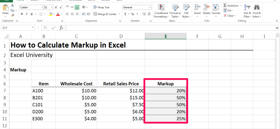
1. Compile the original data table. It is more convenient to work with already named columns. For example, the column where the result of the formula will be displayed can be called “Markup,%”. However, the column heading does not affect the final result and therefore can be anything.
2. Put the “Equals” sign from the keyboard into the required, empty cell of the table array and enter the formula specified in the previous section. For example, enter “(C2-A2) / A2 * 100”. The image below shows the written formula. In parentheses are the names of the cells in which the corresponding values ​​​​of profit and cost of goods are written. In reality, the cells may be different.

3. Press “Enter” on the computer keyboard to complete the formula.
4. Check result. After performing the above manipulations, in the table element where the formula was entered, a specific number should be displayed that characterizes the markup indicator for the product as a percentage.

Important! The markup can be calculated manually to check if the resulting value is correct. If everything is correct, then the prescribed formula must be stretched to the remaining lines of the table array for their automatic filling.

How margin is calculated in MS Excel

For a complete understanding of the topic, it is necessary to consider the margin calculation rule in Microsoft Office Excel. Here, too, there should be no problems even for inexperienced users of the program. For a successful result, you can use a step-by-step algorithm:

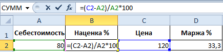
1. Create a spreadsheet to calculate margin. In the initial table array, you can place several parameters for calculation, including the margin.
2. Place the mouse cursor in the corresponding cell of the plate, put the sign “Equal” and write the formula indicated above. For example, let’s write the following expression: “(A2-C2) / C2 * 100”.

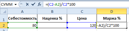
3. Press “Enter” from the keyboard to confirm.
4. Check result. The user must make sure that the previously selected cell has a value that characterizes the margin indicator. For verification, you can manually recalculate the value with the specified indicators. If the answers converge, then the prescribed formula can be extended to the remaining cells of the table array. In this case, the user will save himself from re-filling each required element in the table, saving his own time.

Additional Information! If after writing the formula, the Microsoft Office Excel software generates an error, then the user will need to carefully check the correctness of the characters entered in the expression.

After calculating the markup and margin indicators, you can plot these values ​​​​on the original table in order to visualize the difference between the two dependencies.

How to calculate a percentage value in Excel

If the user needs to understand what number of the total indicator the calculated percentage corresponds to, he must do the following manipulations:

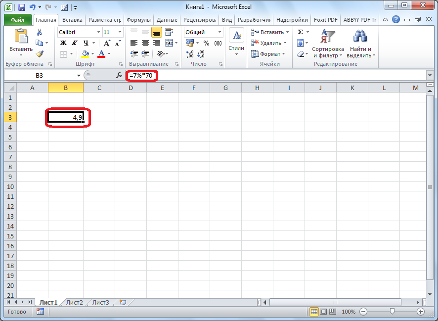
1. In any free cell of the Excel worksheet, write the formula “= percentage value * total amount.” More details in the image below.

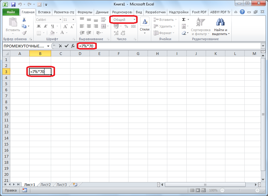
2. Press “Enter” from the PC keyboard to complete the formula.
3. Check result. Instead of a formula, a specific number will appear in the cell, which will be the result of the conversion.

4. You can extend the formula to the remaining rows of the table if the total amount from which the percentage is calculated is the same for the entire condition.

Pay attention! Checking the calculated value is done easily manually using a conventional calculator.

How to calculate percentage of a number in Excel

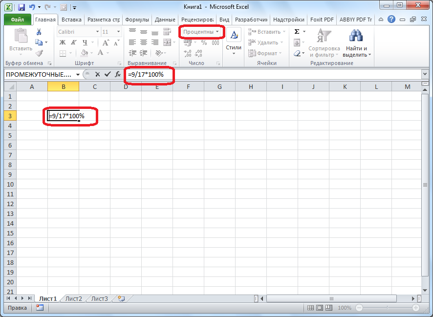
This is the reverse process discussed above. For example, you need to calculate how many percent the number 9 is from the number 17. To cope with the task, you must act as follows:

1. Place the mouse cursor in an empty cell in the Excel worksheet.
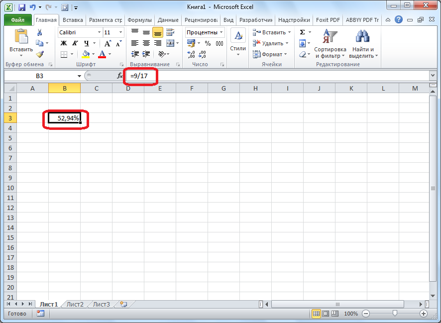
2. Write down the formula “=9/17*100%”.

3. Press “Enter” from the keyboard to complete the formula and see the final result in the same cell. The result should be 52,94%. If necessary, the number of digits after the decimal point can be increased.

Conclusion

Thus, the margin indicator for a particular product in Microsoft Office Excel is calculated using a standard formula. The main thing is to write the expression correctly, indicating the appropriate cells in which the desired values ​​are written. In order to understand this topic well, you need to carefully read the above information.