


Contents
Formatting is one of the main processes when working with a spreadsheet. By applying formatting, you can change the appearance of tabular data, as well as set cell options. It is important to be able to implement it correctly in order to do your work in the program quickly and efficiently. From the article you will learn how to format the table correctly.
Table Formatting
Formatting is a set of actions that is necessary to edit the appearance of a table and the indicators inside it. This procedure allows you to edit the font size and color, cell size, fill, format, and so on. Let’s analyze each element in more detail.
Auto-formatting
Autoformatting can be applied to absolutely any range of cells. The spreadsheet processor will independently edit the selected range, applying the assigned parameters to it. Walkthrough:
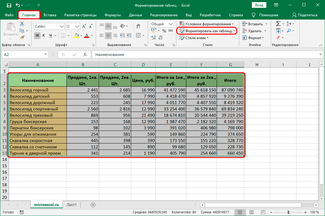
- We select a cell, a range of cells or the entire table.
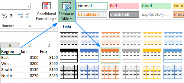
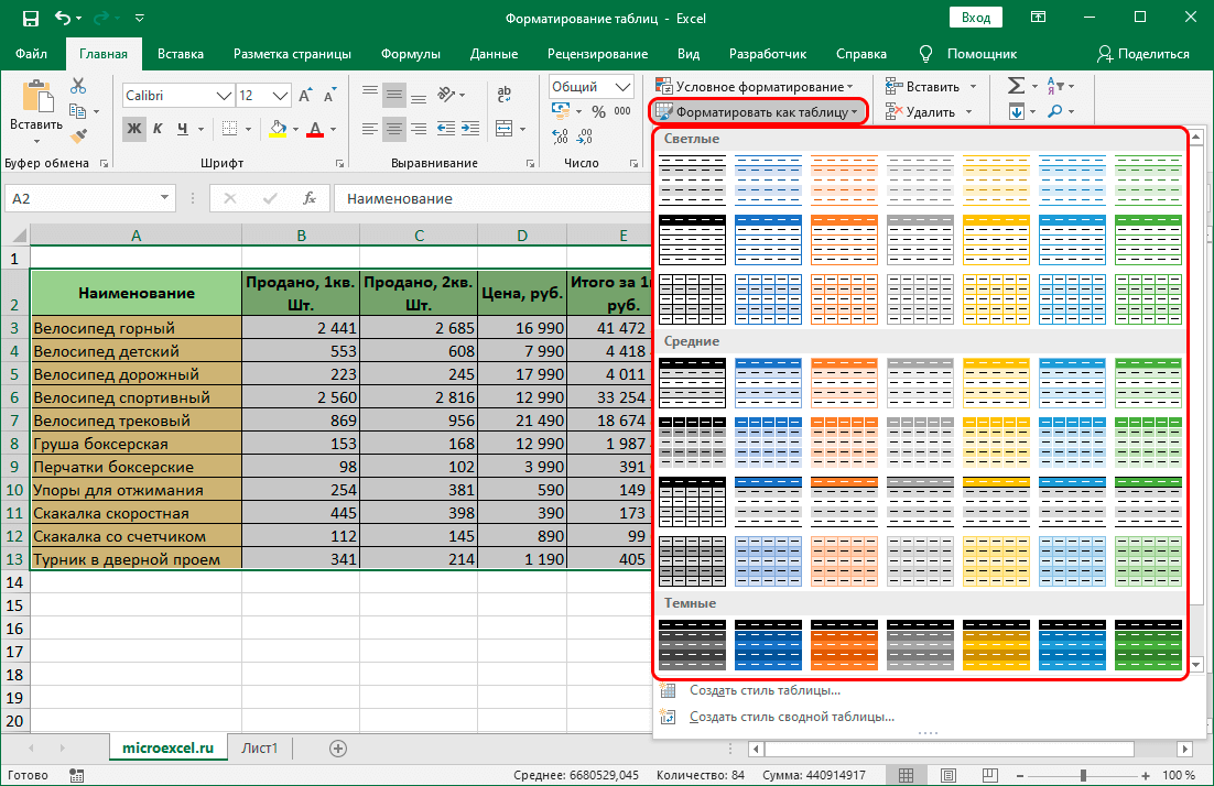
- Go to the “Home” section and click “Format as Table”. You can find this element in the “Styles” block. After clicking, a window with all possible ready-made styles is displayed. You can choose any of the styles. Click on the option you like.
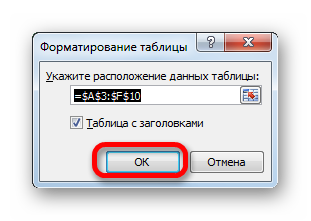
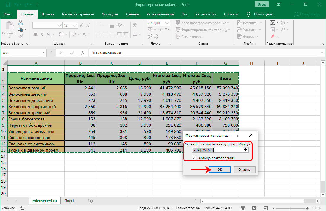
- A small window was displayed on the screen, which requires confirmation of the correctness of the entered range coordinates. If you notice that there is an error in the range, you can edit the data. You need to carefully consider the item “Table with headers.” If the table contains headings, then this property must be checked. After making all the settings, click “OK”.
- Ready! The plate has taken on the appearance of the style you have chosen. At any time, this style can be changed to another.
Switching to formatting
The possibilities of automatic formatting do not suit all users of the spreadsheet processor. It is possible to manually format the plate using special parameters. You can edit the appearance using the context menu or the tools located on the ribbon. Walkthrough:
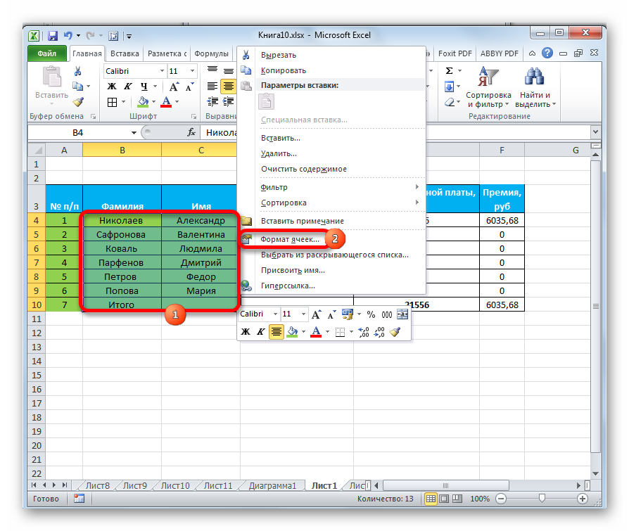
- We make a selection of the necessary editing area. Click on it RMB. The context menu is displayed on the screen. Click on the “Format Cells…” element.
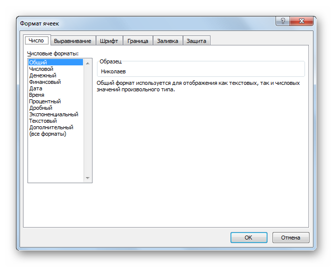
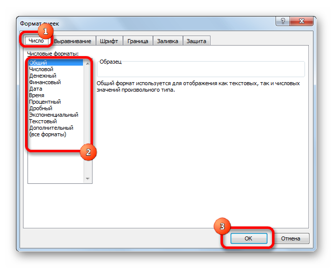
- A box called “Format Cells” appears on the screen. Here you can perform various tabular data editing manipulations.
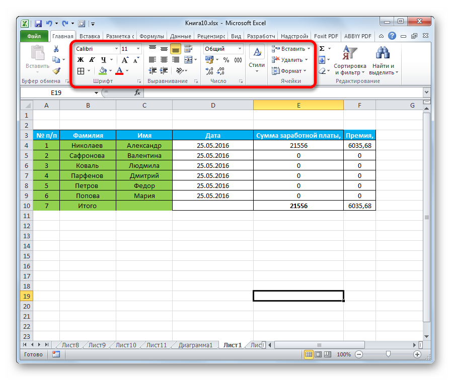
The Home section contains various formatting tools. In order to apply them to your cells, you need to select them, and then click on any of them.
Data Formatting
The cell format is one of the basic formatting elements. This element not only modifies the appearance, but also tells the spreadsheet processor how to process the cell. As in the previous method, this action can be implemented through the context menu or the tools located in the special ribbon of the Home tab.
By opening the “Format Cells” window using the context menu, you can edit the format through the “Number Formats” section, located in the “Number” block. Here you can choose one of the following formats:
- date;
- time;
- common;
- numerical;
- text, etc.
After selecting the required format, click “OK”.
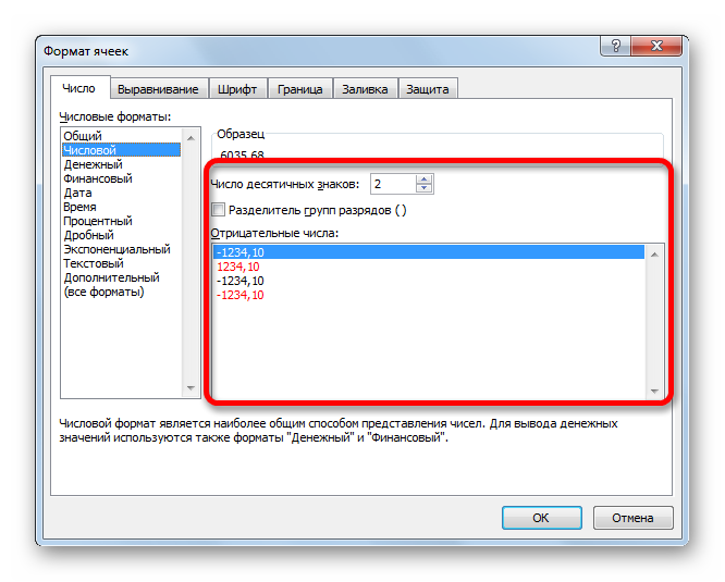
In addition, some formats have additional options. By selecting a number format, you can edit the number of digits after the decimal point for fractional numbers.
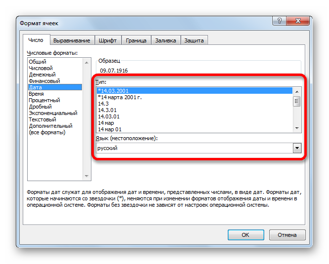
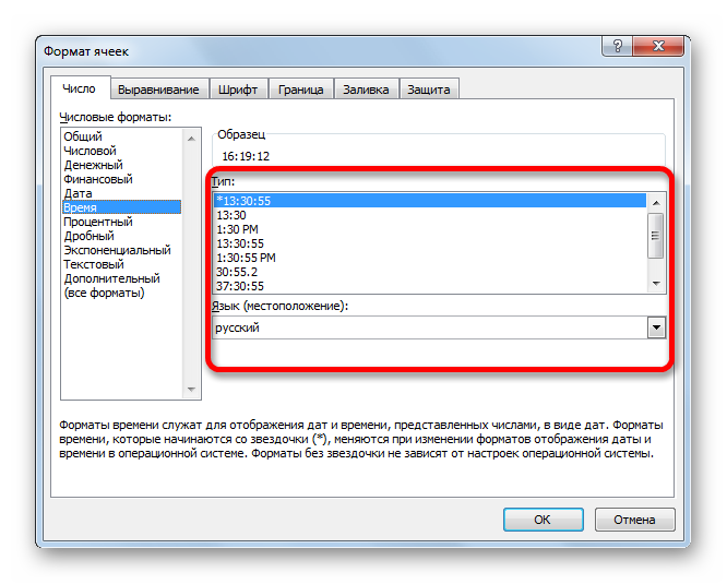
By setting the “Date” format, you can choose how the date will be displayed on the screen. The “Time” parameter has the same settings. By clicking on the “All formats” element, you can view all possible subspecies of editing data in a cell.
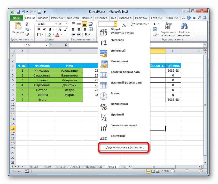
By going to the “Home” section and expanding the list located in the “Number” block, you can also edit the format of a cell or a range of cells. This list contains all the major formats.
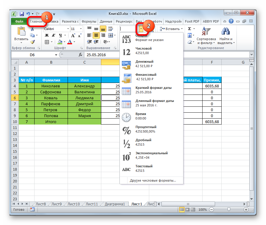
By clicking on the item “Other number formats …” the already known window “Format of cells” will be displayed, in which you can make more detailed settings for the format.
Content alignment
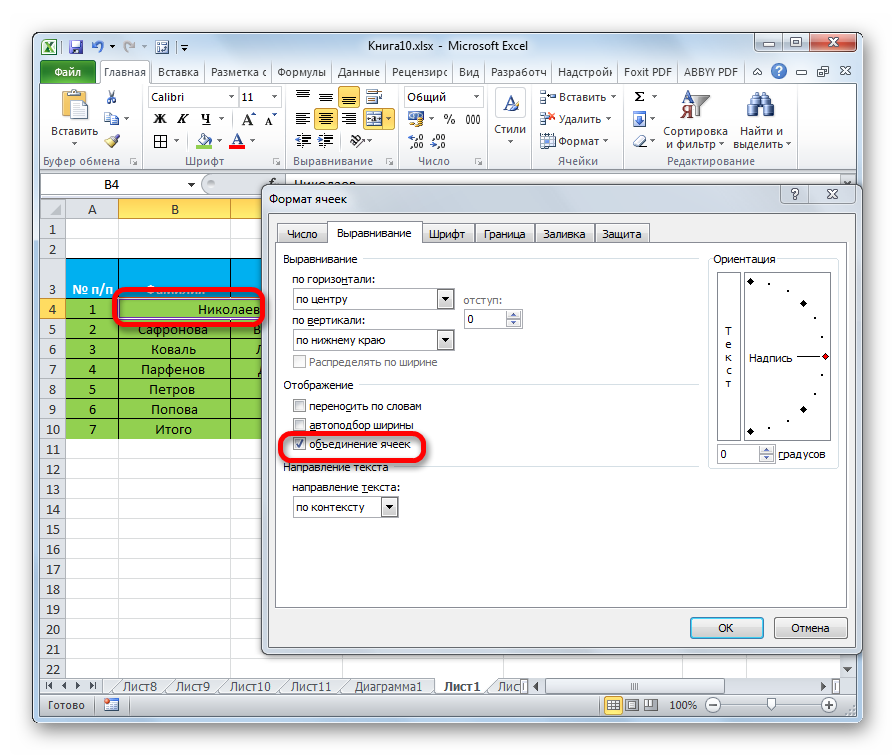
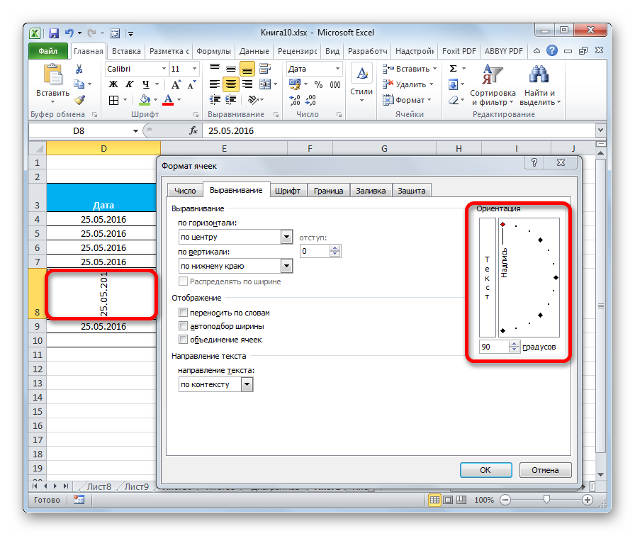
By going to the “Format Cells” box, and then to the “Alignment” section, you can make a number of additional settings to make the appearance of the plate more presentable. This window contains a large number of settings. By checking the box next to one or another parameter, you can merge cells, wrap text by words, and also implement automatic width selection.
In addition, in this section, you can implement the location of the text inside the cell. There is a choice of vertical and horizontal text display.
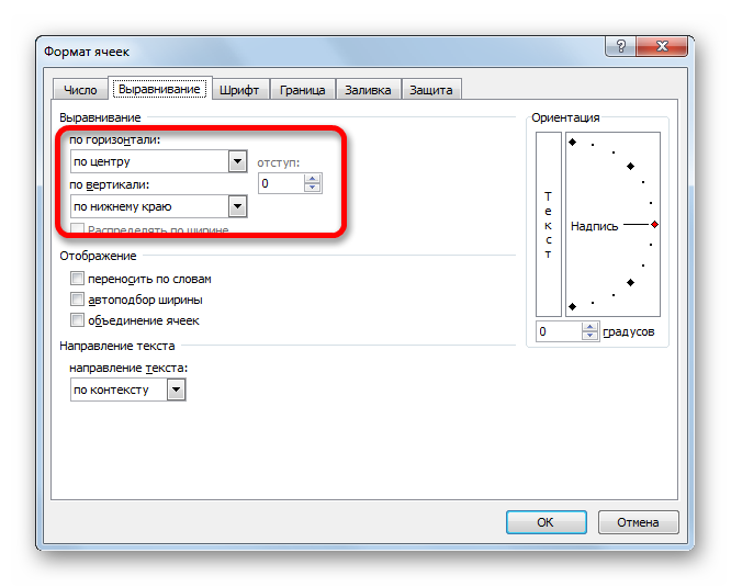
In the “Orientation” section, you can adjust the positioning angle of the text information inside the cell.
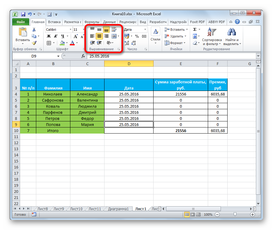
In the “Home” section there is a block of tools “Alignment”. Here, as in the “Format Cells” window, there are data alignment settings, but in a more cropped form.
Font setting
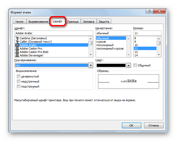
The “Font” section allows you to perform a large set of actions to edit the information in the selected cell or range of cells. Here you can edit the following:
- a type;
- the size;
- Colour;
- style, etc.
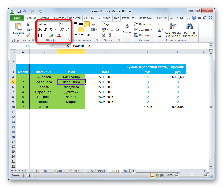
On a special ribbon is a block of tools “Font”, which allows you to perform the same transformations.
Borders and lines
In the “Border” section of the “Format Cells” window, you can customize the line types, as well as set the desired color. Here you can also choose the style of the border: external or internal. It is possible to completely remove the border if it is not needed in the table.
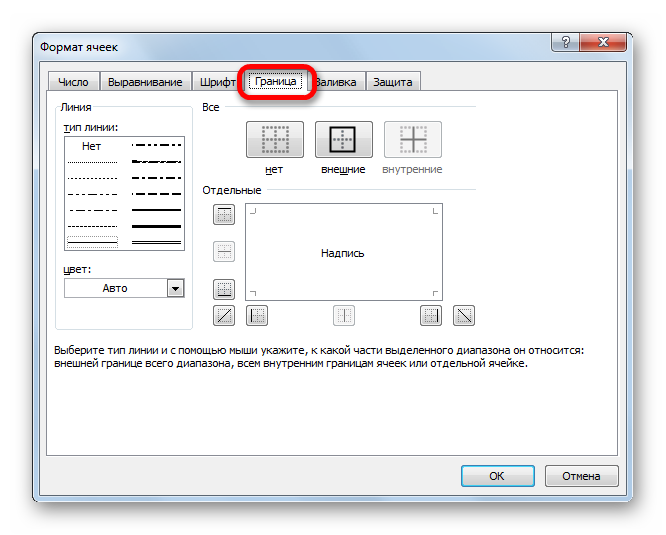
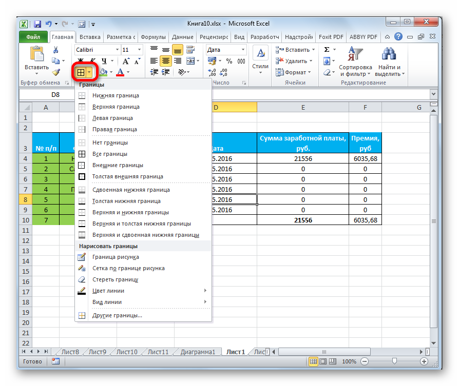
Unfortunately, there are no tools for editing table borders on the top ribbon, but there is a small element that is located in the “Font” block.
Filling cells
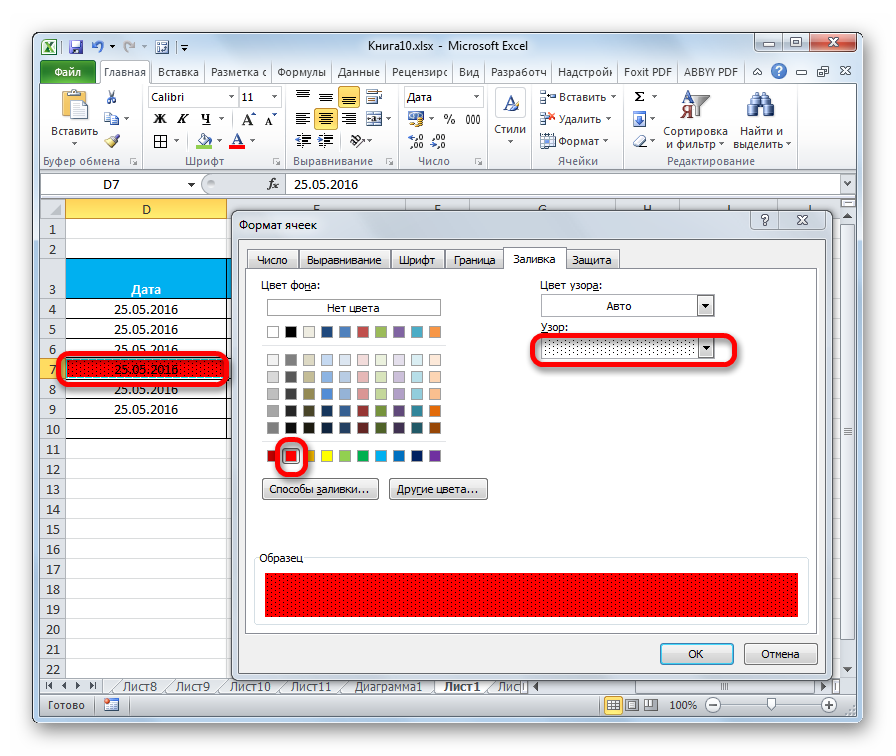
In the “Fill” section of the “Format Cells” box, you can edit the color of the table cells. There is an additional possibility of exhibiting various patterns.
As in the previous element, there is only one button on the toolbar, which is located in the “Font” block.
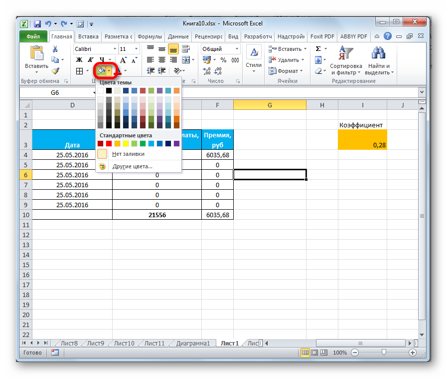
It happens that the user does not have enough standard shades to work with tabular information. In this case, you need to go to the “Other colors …” section through the button located in the “Font” block. After clicking, a window is displayed that allows you to select a different color.
Cell styles
You can not only set the cell style yourself, but also choose from those integrated into the spreadsheet itself. The library of styles is extensive, so each user will be able to choose the right style for themselves.
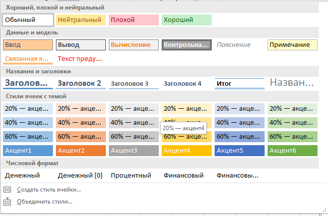
Walkthrough:
- Select the necessary cells to apply the finished style.
- Go to the “Home” section.
- Click “Cell Styles”.
- Choose your favorite style.
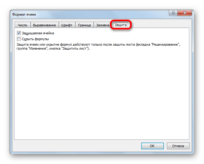
Data protection
Protection also belongs to the realm of formatting. In the familiar “Format Cells” window, there is a section called “Protection”. Here you can set protection options that will prohibit editing the selected range of cells. And also here you can enable hiding formulas.
On the tool ribbon of the Home section, in the Cells block, there is a Format element that allows you to perform similar transformations. By clicking on “Format”, the screen will display a list in which the “Protection” element exists. By clicking on “Protect sheet …”, you can prohibit editing the entire sheet of the desired document.
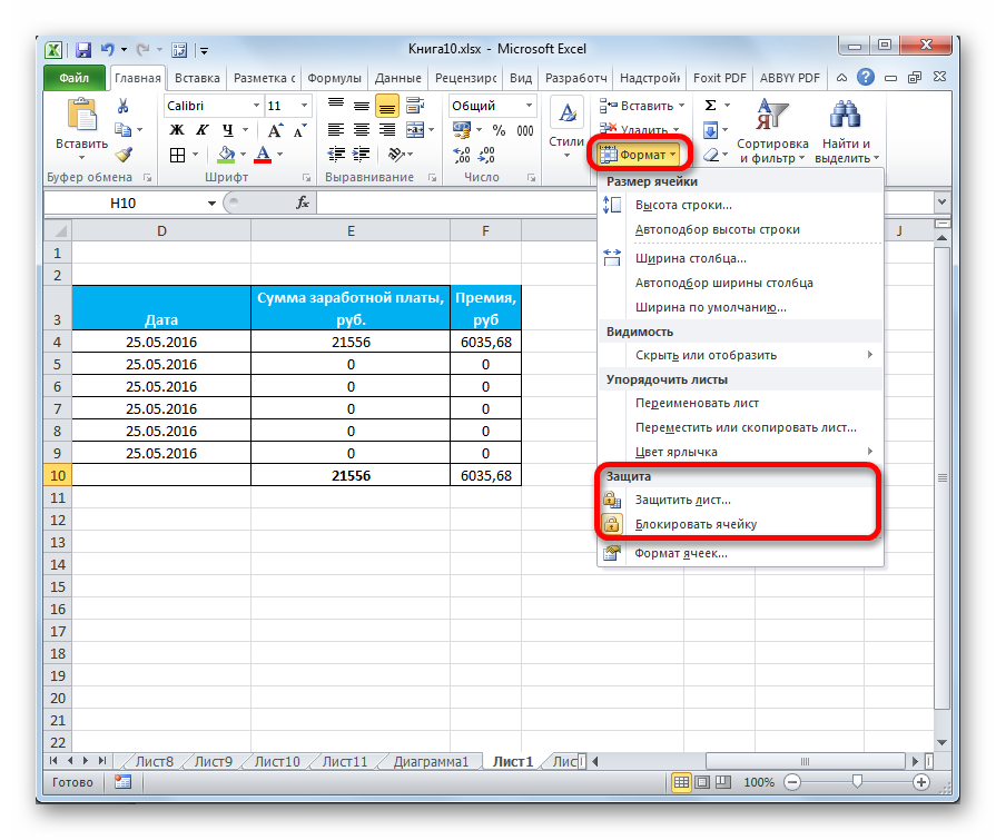
Table themes
In the spreadsheet Excel, as well as the word processor Word, you can choose the theme of the document.
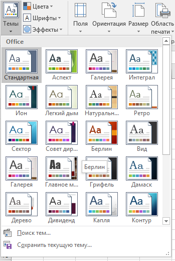
Walkthrough:
- Go to the “Page Layout” tab.
- Click on the “Themes” element.
- Choose one of the ready-made themes.
Transformation into a “Smart Table”
A “smart” table is a special type of formatting, after which the cell array receives certain useful properties that make it easier to work with large amounts of data. After the conversion, the range of cells is considered by the program as a whole element. Using this function saves users from recalculating formulas after adding new rows to the table. In addition, the “Smart” table has special buttons in the headers that allow you to filter the data. The function provides the ability to pin the table header to the top of the sheet. Transformation into a “Smart Table” is performed as follows:
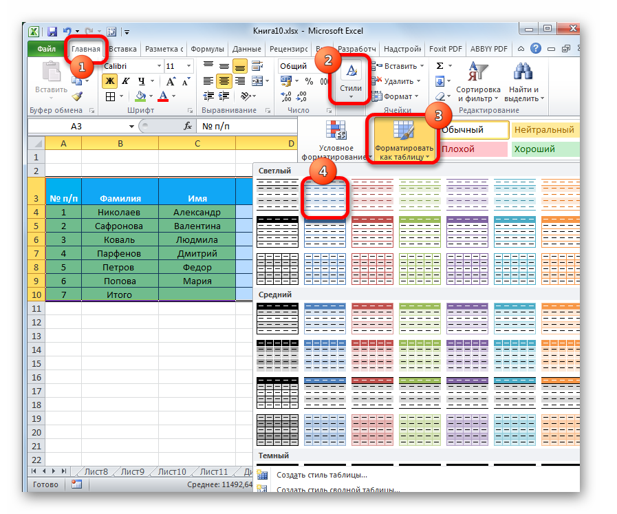
- Select the required area for editing. On the toolbar, select the “Styles” item and click “Format as Table”.
- The screen displays a list of ready-made styles with preset parameters. Click on the option you like.
- An auxiliary window appeared with settings for the range and display of titles. We set all the necessary parameters and click the “OK” button.
- After making these settings, our tablet turned into a Smart Table, which is much more convenient to work with.
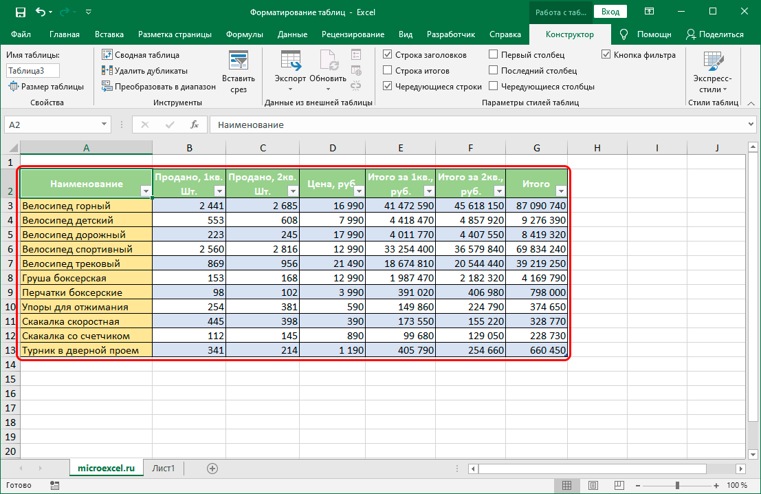
Table Formatting Example
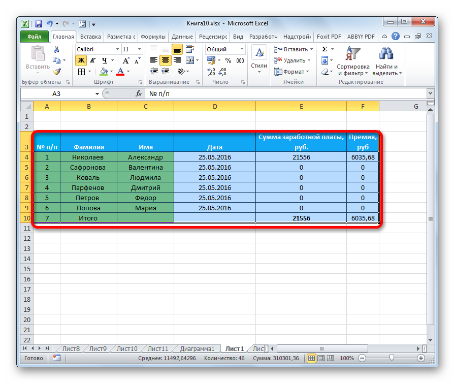
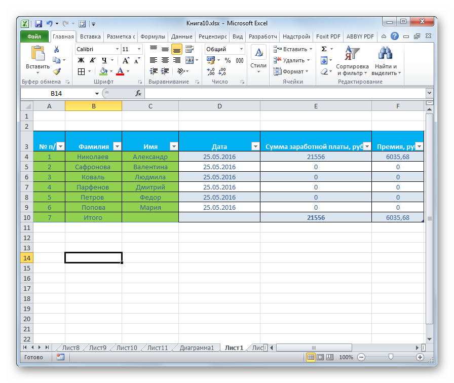
Let’s take a simple example of how to format a table step by step. For example, we have created a table like this:
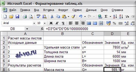
Now let’s move on to its detailed editing:
- Let’s start with the title. Select the range A1 … E1, and click on “Merge and move to the center.” This item is located in the “Formatting” section. The cells are merged and the inner text is center aligned. Set the font to “Arial”, the size to “16”, “Bold”, “Underlined”, the font shade to “Purple”.
- Let’s move on to formatting the column headings. Select cells A2 and B2 and click “Merge Cells”. We perform similar actions with cells A7 and B7. We set the following data: font – “Arial Black”, size – “12”, alignment – “Left”, font shade – “Purple”.
- We make a selection of C2 … E2, while holding “Ctrl”, we make a selection of C7 … E7. Here we set the following parameters: font – “Arial Black”, size – “8”, alignment – “Centered”, font color – “Purple”.
- Let’s move on to editing posts. We select the main indicators of the table – these are cells A3 … E6 and A8 … E8. We set the following parameters: font – “Arial”, “11”, “Bold”, “Centered”, “Blue”.
- Align to the left edge B3 … B6, as well as B8.
- We expose the red color in A8 … E8.
- We make a selection of D3 … D6 and press RMB. Click “Format Cells…”. In the window that appears, select the numeric data type. We perform similar actions with cell D8 and set three digits after the decimal point.
- Let’s move on to formatting the borders. We make a selection of A8 … E8 and click “All Borders”. Now select “Thick Outer Border”. Next, we make a selection of A2 … E2 and also select “Thick outer border”. In the same way, we format A7 … E7.
- We do color setting. Select D3…D6 and assign a light turquoise hue. We make a selection of D8 and set a light yellow tint.
- We proceed to the installation of protection on the document. We select cell D8, right-click on it and click “Format Cells”. Here we select the “Protection” element and put a checkmark next to the “Protected cell” element.
- We move to the main menu of the spreadsheet processor and go to the “Service” section. Then we move to “Protection”, where we select the element “Protect Sheet”. Setting a password is an optional feature, but you can set it if you wish. Now this cell cannot be edited.
In this example, we examined in detail how you can format a table in a spreadsheet step by step. The result of formatting looks like this:
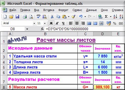
As we can see, the sign has changed drastically from the outside. Her appearance has become more comfortable and presentable. By similar actions, you can format absolutely any table and put protection on it from accidental editing. The manual formatting method is much more efficient than using predefined styles, since you can manually set unique parameters for any type of table.
Conclusion
The spreadsheet processor has a huge number of settings that allow you to format data. The program has convenient built-in ready-made styles with set formatting options, and through the “Format Cells” window, you can implement your own settings manually.