


Contents
What are dynamic arrays
In September 2018, Microsoft released an update that adds a completely new tool to Microsoft Excel: Dynamic Arrays and 7 new functions for working with them. These things, without exaggeration, radically change all the usual technique of working with formulas and functions and concern, literally, every user.
Consider a simple example to explain the essence.
Suppose we have a simple table with data on city-months. What will happen if we select any empty cell on the right of the sheet and enter into it a formula that links not to one cell, but immediately to a range?
In all previous versions of Excel, after clicking on Enter we would get the contents of only one first cell B2. How else?
Well, or it would be possible to wrap this range in some kind of aggregating function like =SUM(B2:C4) and get a grand total for it.
If we needed more complex operations than a primitive sum, such as extracting unique values or Top 3, then we would have to enter our formula as an array formula using a keyboard shortcut Ctrl+Shift+Enter.
Now everything is different.
Now after entering such a formula, we can simply click on Enter – and get as a result immediately all the values uXNUMXbuXNUMXbto which we referred:
This is not magic, but the new dynamic arrays that Microsoft Excel now has. Welcome to the new world 🙂
Features of working with dynamic arrays
Technically, our entire dynamic array is stored in the first cell G4, filling the required number of cells to the right and down with its data. If you select any other cell in the array, then the link in the formula bar will be inactive, showing that we are in one of the “child” cells:
An attempt to delete one or more “child” cells will not lead to anything – Excel will immediately recalculate and fill them.
At the same time, we can safely refer to these “child” cells in other formulas:
If you copy the first cell of an array (for example, from G4 to F8), then the entire array (its references) will move in the same direction as in regular formulas:
If we need to move the array, then it will be enough to move (with the mouse or a combination of Ctrl+X, Ctrl+V), again, only the first main cell G4 – after it, it will be transferred to a new place and our entire array will be expanded again.
If you need to refer somewhere else on the sheet to the created dynamic array, then you can use the special character # (“pound”) after the address of its leading cell:
For example, now you can easily make a dropdown list in a cell that refers to the created dynamic array:
Dynamic array errors
But what happens if there is not enough space to expand the array, or if there are cells already occupied by other data in its path? Meet a fundamentally new type of errors in Excel – #TRANSFER! (#SPILL!):
As always, if we click on the icon with a yellow diamond and an exclamation mark, we will get a more detailed explanation of the source of the problem and we can quickly find interfering cells:
Similar errors will occur if the array goes off the sheet or hits a merged cell. If you remove the obstacle, then everything will immediately be corrected on the fly.
Dynamic arrays and smart tables
If the dynamic array points to a “smart” table created by a keyboard shortcut Ctrl+T or by Home – Format as a table (Home — Format as Table), then it will also inherit its main quality – auto-sizing.
When adding new data to the bottom or to the right, the smart table and dynamic range will also automatically stretch:
However, there is one limitation: we cannot use a dynamic range reference in forumulas inside a smart table:
Dynamic arrays and other Excel features
Okay, you say. All this is interesting and funny. No need, as before, to manually stretch the formula with a reference to the first cell of the original range down and to the right and all that. And that’s all?
Not quite.
Dynamic arrays are not just another tool in Excel. Now they are embedded in the very heart (or brain) of Microsoft Excel – its calculation engine. This means that other Excel formulas and functions familiar to us now also support working with dynamic arrays. Let’s take a look at a few examples to give you an idea of the depth of the changes that have taken place.
Transpose
To transpose a range (swap rows and columns) Microsoft Excel has always had a built-in function TRANSP (TRANSPOSE). However, in order to use it, you must first correctly select the range for the results (for example, if the input was a range of 5×3, then you must have selected 3×5), then enter the function and press the combination Ctrl+Shift+Enter, because it could only work in array formula mode.
Now you can just select one cell, enter the same formula into it and click on the normal Enter – dynamic array will do everything by itself:
Multiplication table
This is the example I used to give when I was asked to visualize the benefits of array formulas in Excel. Now, to calculate the entire Pythagorean table, it is enough to stand in the first cell B2, enter there a formula that multiplies two arrays (vertical and horizontal set of numbers 1..10) and simply click on Enter:
Gluing and case conversion
Arrays can not only be multiplied, but also glued together with the standard operator & (ampersand). Suppose we need to extract the first and last name from two columns and correct the jumping case in the original data. We do this with one short formula that forms the entire array, and then we apply the function to it PROPNACH (PROPER)to tidy up the register:
Conclusion Top 3
Suppose we have a bunch of numbers from which we want to derive the top three results, arranging them in descending order. Now this is done by one formula and, again, without any Ctrl+Shift+Enter like before:
If you want the results to be placed not in a column, but in a row, then it is enough to replace the colons (line separator) in this formula with a semicolon (element separator within one line). In the English version of Excel, these separators are semicolons and commas, respectively.
VLOOKUP extracting multiple columns at once
Functions VPR (VLOOKUP) now you can pull values not from one, but from several columns at once – just specify their numbers (in any desired order) as an array in the third argument of the function:
OFFSET function returning a dynamic array
One of the most interesting and useful (after VLOOKUP) functions for data analysis is the function DISPOSAL (OFFSET), to which I devoted at one time a whole chapter in my book and an article here. The difficulty in understanding and mastering this function has always been that it returned an array (range) of data as a result, but we could not see it, because Excel still didn’t know how to work with arrays out of the box.
Now this problem is in the past. See how now, using a single formula and a dynamic array returned by OFFSET, you can extract all rows for a given product from any sorted table:
Let’s take a look at her arguments:
- A1 – starting cell (reference point)
- ПОИСКПОЗ(F2;A2:A30;0) – calculation of the shift from the starting cell down – to the first found cabbage.
- 0 – shift of the “window” to the right relative to the starting cell
- СЧЁТЕСЛИ(A2:A30;F2) – calculation of the height of the returned “window” – the number of lines where there is cabbage.
- 4 — size of the “window” horizontally, i.e. output 4 columns
New Functions for Dynamic Arrays
In addition to supporting the dynamic array mechanism in old functions, several completely new functions have been added to Microsoft Excel, sharpened specifically for working with dynamic arrays. In particular, these are:
- GRADE (SORT) – sorts the input range and produces a dynamic array on the output
- SORTPO (SORTBY) – can sort one range by values from another
- FILTER (FILTER) – retrieves rows from the source range that meet the specified conditions
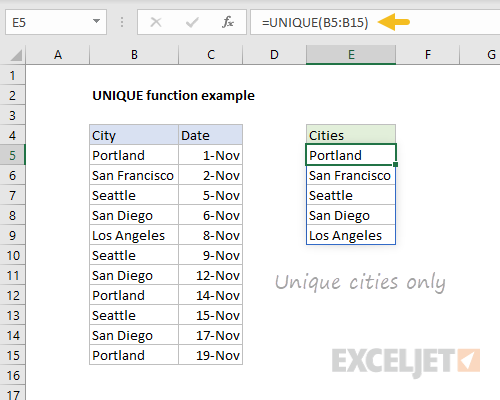
- UNIK (UNIQUE) – extracts unique values from a range or removes duplicates
- SLMASSIVE (RANDARRAY) – generates an array of random numbers of a given size
- AFTERBIRTH (SEQUENCE) — forms an array from a sequence of numbers with a given step
More about them – a little later. They are worth a separate article (and not one) for thoughtful study 🙂
Conclusions
If you have read everything written above, then I think you already realize the scale of the changes that have taken place. So many things in Excel can now be done easier, easier and more logical. I must admit that I am a little shocked at how many articles will now have to be corrected here, on this site and in my books, but I am ready to do this with a light heart.
Summing up the results, плюсы dynamic arrays, you can write the following:
- You can forget about the combination Ctrl+Shift+Enter. Excel now sees no difference between “regular formulas” and “array formulas” and treats them the same way.
- About the function SUMPRODUCT (SUMPRODUCT), which was previously used to enter array formulas without Ctrl+Shift+Enter you can also forget – now it’s easy enough SUM и Enter.
- Smart tables and familiar functions (SUM, IF, VLOOKUP, SUMIFS, etc.) now also fully or partially support dynamic arrays.
- There is backward compatibility: if you open a workbook with dynamic arrays in an old version of Excel, they will turn into array formulas (in curly braces) and continue to work in the “old style”.
Found some number minuses:
- You cannot delete individual rows, columns or cells from a dynamic array, i.e. it lives as a single entity.
- You cannot sort a dynamic array in the usual way through Data – Sorting (Data — Sort). There is now a special function for this. GRADE (SORT).
- A dynamic range cannot be turned into a smart table (but you can make a dynamic range based on a smart table).
Of course, this is not the end, and I’m sure Microsoft will continue to improve this mechanism in the future.
Where can I download?
And finally, the main question 🙂
Microsoft first announced and showed a preview of dynamic arrays in Excel back in September 2018 at a conference Ignite. In the next few months, there was a thorough testing and running-in of new features, first on cats employees of Microsoft itself, and then on volunteer testers from the circle of Office Insiders. This year, the update that adds dynamic arrays began to be gradually rolled out to regular Office 365 subscribers. For example, I only received it in August with my Office 365 Pro Plus (Monthly Targeted) subscription.
If your Excel does not yet have dynamic arrays, but you really want to work with them, then there are the following options:
- If you have an Office 365 subscription, you can simply wait until this update reaches you. How quickly this happens depends on how often updates are delivered to your Office (once a year, once every six months, once a month). If you have a corporate PC, you can ask your administrator to set up updates to be downloaded more often.
- You can join the ranks of those Office Insiders test volunteers – then you will be the first to receive all the new features and functions (but there is a chance of increased buggy in Excel, of course).
- If you do not have a subscription, but a boxed standalone version of Excel, then you will have to wait until the release of the next version of Office and Excel in 2022, at least. Users of such versions receive only security updates and bug fixes, and all the new “goodies” now go only to Office 365 subscribers. Sad but true 🙂
In any case, when dynamic arrays appear in your Excel – after this article, you will be ready for it 🙂
- What are array formulas and how to use them in Excel
- Window (range) summation using the OFFSET function
- 3 Ways to Transpose a Table in Excel