


Contents
A logical function is a type of function that can return one of the possible values - true if the cell contains values that meet certain criteria and false if this does not happen. Logic functions are used to program spreadsheets in order to achieve unloading yourself from frequently repetitive actions.
In addition, logical functions can be used to check to what extent the contents of a cell meet certain criteria. Other boolean values can also be checked.
Comparison Operators
Each expression contains comparison operators. They are as follows:
- = – value 1 is equal to value 2.
- > – value 1 is greater than value 2.
- < – ачение 1 еньше ачения 2.
- >= value 1 or identical to value 2 or greater.
- <= ачение 1 еньше ачению 2 идентично ему.
- <> value 1 or greater than value 2 or less.
As a consequence, Excel returns one of two possible results: true (1) or false (2).
To use logical functions, it is necessary, in all possible cases, to specify a condition that contains one or more operators.
True function
Для использования этой функции не нужно указывать никаких аргументов, и она всегда возвращает «Истина» (что соответствует цифре 1 двоичной системы счисления).
Formula Example − =TRUE().
False function
The function is completely similar to the previous one, only the result returned by it is “False”. The easiest formula where you can use this function is the following =ЛОЖЬ().
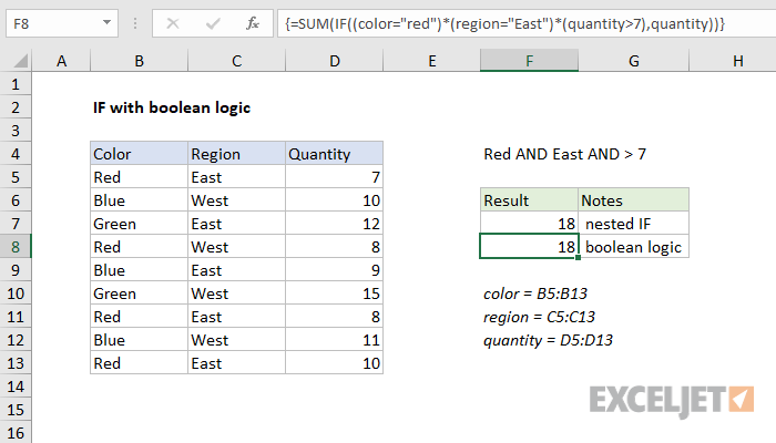
AND function
The purpose of this formula is to return the value “True” when each of the arguments matches a certain value or certain criteria, which are described above. If suddenly there is a discrepancy between one of the criteria required, then the value “False” is returned.
Boolean cell references are also used as function parameters. The maximum number of arguments that can be used is 255. But the mandatory requirement is the presence of at least one of them in brackets.
| И | Truth | False |
| Truth | Truth | False |
| False | False | False |
The syntax for this function is:
=AND(Boolean1; [Boolean2];…)
На данном скриншоте видно, что каждый аргумент передает истинное значение, поэтому в результате использования этой формулы можно получить соответствующий результат.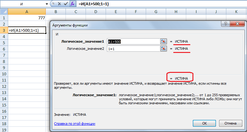
“Or” function
Checks multiple values against certain criteria. If any of them matches, then the function returns the true value (1). The maximum number of arguments in this situation is also 255, and it is mandatory to specify one function parameter.
Speaking of function OR, then in the case of it the truth table will be as follows.
| OR | Truth | False |
| Truth | Truth | Truth |
| False | Truth | False |
The formula syntax is as follows:
=OR(Boolean 1; [Boolean 2];…)
Just as in the previous and following cases, each argument must be separated from the other with a semicolon. If we refer to the example above, then each parameter returns “True” there, so if it is necessary to use the “OR” function when accessing this range, then the formula will return “True” until one of the parameters meets a certain criterion.
“No” function
It returns those values that are opposite to the one originally set. That is, when passing the value “True” as a function parameter, “False” will be returned. If no match is found, then “True”.
The result that will be returned depends on what initial argument is received by the function. If, for example, the “AND” function is used together with the “NOT” function, then the table will be as follows.
| NOT(and()) | TRUE | LYING |
| TRUE | LYING | TRUE |
| LYING | TRUE | TRUE |
When using the “Or” function in combination with the “Not” function, the table will look like this.
| NOT (OR()) | TRUE | LYING |
| TRUE | LYING | LYING |
| LYING | LYING | TRUE |
The syntax for this function is very simple: =НЕ(принимаемое логическое значение).
If
This feature can rightly be called one of the most popular. It checks a particular expression against a particular condition. The result is affected by the truth or falsity of a given statement.
If we talk specifically about this function, then its syntax will be somewhat more complicated.
=IF(Boolean_expression,[Value_if_true],[Value_if_false])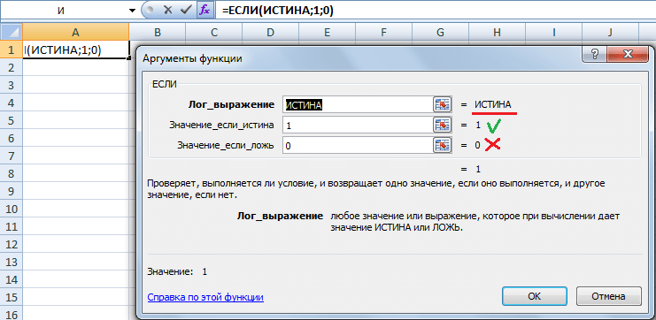
Let’s take a closer look at the example that was shown in the screenshot above. Here, the first parameter is the function TRUE, which is checked by the program. Based on the results of such a check, the second argument is returned. The third one goes down.
User can nest one function IF to another. This must be done in cases where, as a result of one check for compliance with a certain condition, it is necessary to do another one.
For example, there are several credit cards that have numbers that begin with the first four digits that characterize the payment system servicing the card. That is, there are two options – Visa and Mastercard. To check the card type, you need to use this formula with two nested IF.
=IF(LEFT(A2)=”4″, “Visa”,IF(LEFT(A1111)=”2″,”Master Card”,”card not defined”))
If you don’t know what the function means LEVSIMV, then it writes to the cell part of the line of text on the left. The user in the second argument to this function specifies the number of characters that Excel should select from the left. It is used to check if the first four digits of a credit card number begin with 1111. If the result is true, “Visa” is returned. If the condition is false, then the function is used IF.
Similarly, you can achieve decent nesting and check the contents of a cell or range for compliance with several conditions.
ERROR function
Needed in order to determine if there is an error. If yes, then the value of the second argument is returned. If everything is in order, then the first. In total, the function has two arguments, each of which is required.
This formula has the following syntax:
=IFERROR(value;value_if_error)
How can the function be used?
In the example below, you can see the error in the first function argument. Therefore, the formula returns the answer that division by zero is prohibited. The first parameter of the function can be any other formulas. A person can independently decide what content can be there.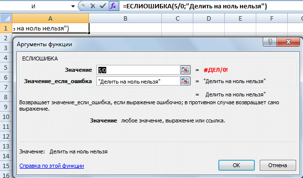
How boolean functions can be used in practice
Task 1
Before the person set the goal to carry out a revaluation of commodity balances. If the product is stored for more than 8 months, it is necessary to reduce its cost by half.
Initially, you need to create such a table.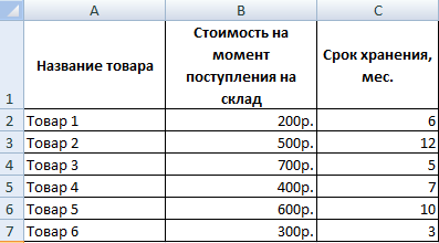
To achieve this goal, you need to use the function IF. In the case of our example, this formula will look like this:
=ЕСЛИ(C2>=8;B2/2;B2)
The boolean expression contained in the first argument of the function is composed using the > and = operators. In simple words, initially the criterion is as follows: if the cell value is greater than or equal to 8, the formula supplied in the second argument is executed. In terminological terms, if the first condition is true, then the second argument is executed. If false – the third.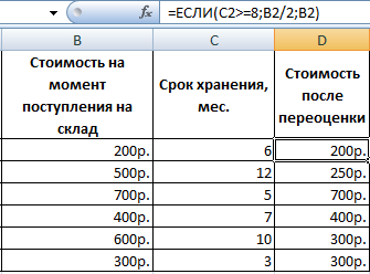
The complexity of this task can be increased. Suppose that we are faced with the task of using the logical function AND. In this case, the condition will take the following form: if the product is stored for more than 8 months, then its price must be reset twice. If it has been on sale for more than 5 months, then it must be reset by 1,5 times.
In this case, you need to enter the following string in the formula input field.
=ЕСЛИ(И(C2>=8);B2/2;ЕСЛИ(И(C2>=5);B2/1,5;B2))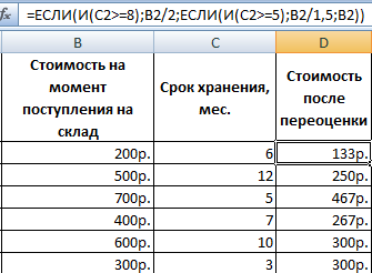
Function IF allows text strings in arguments if required.
Task 2
Suppose, after the product was discounted, it began to cost less than 300 rubles, then it must be written off. The same must be done if it has lain without being sold for 10 months. In this situation, any of these options is acceptable, so it is logical to use the function OR и IF. The result is the following line.
=ЕСЛИ(ИЛИ(D2<300;C2>=10);»списан»;»»)
If the logical operator was used when writing the condition OR, then it must be decoded as follows. If cell C2 contains the number 10 or more, or if cell D2 contains a value less than 300, then the value “written off” must be returned in the corresponding cell.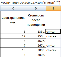
If the condition is not met (that is, it turns out to be false), then the formula automatically returns an empty value. Thus, if the product was sold earlier or is in stock less than necessary, or it was discounted to a value less than the threshold value, then an empty cell remains.
It is allowed to use other functions as arguments. For example, the use of mathematical formulas is acceptable.
Task 3
Suppose there are several students who take several exams before entering the gymnasium. As a passing score, there is a score of 12. And in order to enter, it is imperative that there be at least 4 points in mathematics. As a result, Excel should generate a receipt report.
First you need to build the following table.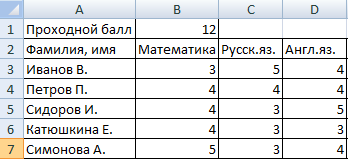
Our task is to compare the sum of all grades with the passing score, and in addition to make sure that the grade in mathematics is below 4. And in the column with the result, you must indicate “accepted” or “no”.
We need to enter the following formula.
=ЕСЛИ(И(B3>=4;СУММ(B3:D3)>=$B$1);»принят»;»нет»)
Using the logical operator И it is necessary to check how true these conditions are. And to determine the final score, you need to use the classic function SUM.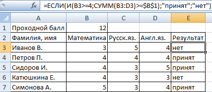
Thus, using the function IF you can solve many different problems, so it is one of the most common.
Task 4
Suppose we are faced with the need to understand how much goods cost after valuation as a whole. If the cost of a product is lower than the average value, then it is necessary to write off this product.
To do this, you can use the same table that was given above.
To solve this problem, you need to use the following formula.
=IF(D2
In the expression given in the first argument, we used the function AVERAGEA that specifies the arithmetic mean of a particular data set. In our case, this is the range D2:D7.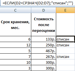
Task 5
In this case, let’s say we need to determine average sales. To do this, you need to create such a table.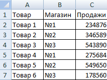
Next, you should calculate the average value of those cells whose contents meet a certain criterion. Thus, both a logical and a statistical solution must be used. Under the table above, you need to create an auxiliary table in which the results will be displayed.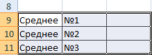
This task can be solved using just one function.
=СРЗНАЧЕСЛИ($B$2:$B$7;B9;$C$2:$C$7)
The first argument is the range of values to be checked. The second specifies the condition, in our case it is cell B9. But as the third argument, the range is used, which will be used in order to calculate the arithmetic mean.
Function HEARTLESS allows you to compare the value of cell B9 with those values that are located in the range B2:B7, which lists the store numbers. If the data matches, then the formula calculates the arithmetic mean of the C2:C7 range.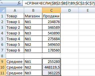
Conclusions
Logic functions are needed in different situations. There are many kinds of formulas that can be used to test for certain conditions. As seen above, the main function is IF, но существует множество других, которые можно использовать в различных ситуациях.
Several examples were also given of how logic functions can be used in real situations.
There are many more aspects of the use of logical functions, but it is difficult to consider them all within the framework of one, even a large, article. There is no limit to perfection, so you can always look for new applications of already known formulas.