


Contents
Excel is considered by many to be a spreadsheet program. Therefore, the question of how to create and work with tables may seem strange at first glance. But few people know what is the main difference between Excel and spreadsheets. In addition, this component of the Microsoft Office package is not always interaction with spreadsheets. Moreover, the main task of Excel is the processing of information that can be presented in different forms. Also in tabular form.
Or a situation may arise when it is necessary to select a separate range for the table and format it accordingly. In general, there are a huge number of possibilities for using tables, so let’s look at them in more detail.
The concept of smart tables
There is still a difference between an Excel sheet and a smart spreadsheet. The first is simply an area containing a certain number of cells. Some of them may be filled with certain information, while others are empty. But there is no fundamental difference between them from a technical point of view.
But an Excel spreadsheet is a fundamentally different concept. It is not limited to a range of data, it has its own properties, a name, a certain structure and a huge number of advantages.
Therefore, you can select a separate name for the Excel table – “Smart Table” or Smart Table.
Create a smart table
Suppose we have created a data range with sales information.
It’s not yet a table. To turn a range into it, you need to select it and find the “Insert” tab and there find the “Table” button in the block of the same name.
A small window will appear. In it, you can adjust the set of cells that you want to turn into a table. In addition, you must specify that the first line contains the column headings. You can also use the keyboard shortcut Ctrl + T to bring up the same dialog box.
In principle, nothing needs to be changed in most cases. After the action is confirmed by pressing the “OK” button, the previously selected range will immediately become a table.
Before directly setting its properties, you need to understand how the program itself sees the table. After that, a lot of things will become clear.
Understanding Excel Table Structure
All tables have a specific name displayed on a special Design tab. It is shown right after selection of any cell. By default, the name takes the form “Table 1” or “Table 2”, and respectively.
If you need to have several tables in one document, it is recommended to give them such names so that later you can understand what information is contained where. In the future, it will then become much easier to interact with them, both for you and for people viewing your document.
In addition, named tables can be used in Power Query or a number of other add-ins.
Let’s call our table “Report”. The name can be seen in a window called the name manager. To open it, you need to go along the following path: Formulas – Defined Names – Name Manager.
It is also possible to manually enter the formula, where you can also see the table name.
But the most amusing thing is that Excel is able to simultaneously see the table in several sections: in its entirety, as well as in individual columns, headings, totals. Then the links will look like this.
In general, such constructions are given only for the purpose of more accurate orientation. But there is no need to memorize them. They are automatically displayed in tooltips that appear after selecting Table and how the square brackets will be opened. To insert them, you must first enable the English layout.
The desired option can be found using the Tab key. Do not forget to close all the brackets that are in the formula. Squares are no exception here.
If you want to sum the contents of the entire column with sales, you must write the following formula:
=SUM(D2:D8)
After that, it will automatically turn into =SUM(Report[Sales]). In simple words, the link will lead to a specific column. Convenient, agree?
Thus, any chart, formula, range, where a smart table will be used to take data from it, will use up-to-date information automatically.
Now let’s talk in more detail about which tables can have properties.
Excel Tables: Properties
Each created table can have multiple column headings. The first line of the range then serves as the data source.
In addition, if the table size is too large, when scrolling down, instead of the letters indicating the corresponding columns, the names of the columns are displayed. This will be to the liking of the user, since it will not be necessary to fix the areas manually.
It also includes an autofilter. But if you don’t need it, you can always turn it off in the settings.
Also, all values that are written immediately below the last cell of the table column are attached to it themselves. Therefore, they can be found directly in any object that uses data from the first column of the table in its work.
At the same time, new cells are formatted for the design of the table, and all formulas specific to this column are automatically written into them. In simple words, to increase the size of the table and expand it, just enter the correct data. Everything else will be added by the program. The same goes for new columns.
If a formula is entered into at least one cell, then it automatically spreads to the entire column. That is, you do not need to manually fill in the cells, everything will happen automatically, as shown in this animated screenshot.
All of these features are good. But you can customize the table yourself and expand its functionality.
Table setup
First you need to open the “Designer” tab, where the table parameters are located. You can customize them by adding or clearing specific checkboxes located in the “Table Style Options” group.
The following options are provided:
- Add or remove a header row.
- Add or remove a row with totals.
- Make lines alternate.
- Highlight extreme columns in bold.
- Enables or disables striped line fills.
- Disable autofilter.
You can also set a different format. This can be done using the options located in the Table Styles group. Initially, the format is different from the one above, but in which case you can always customize the look you want.
You can also find the “Tools” group, where you can create a pivot table, delete copies, and convert the table to a standard range.
But the most entertaining feature is the creation of slices.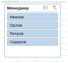
A slice is a type of filter that is displayed in a separate graphic element. To insert it, you need to click on the “Insert Slicer” button of the same name, and then select the columns that you want to leave.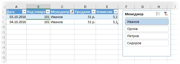
That’s it, now a panel appears, which lists all the unique values contained in the cells of this column.
To filter the table, you must select the category that is most interesting at the moment.
Multiple categories can be selected using a slicer. To do this, you must press the Ctrl key or click on the button in the upper right corner to the left of removing the filter before starting the selection.
To set parameters directly on the ribbon, you can use the tab of the same name. With its help, it is possible to edit various properties of the slice: appearance, button size, quantity, and so on.
Key Limitations of Smart Tables
Despite the fact that Excel spreadsheets have many advantages, the user will still have to put up with some disadvantages:
- The views don’t work. In simple words, there is no way to remember certain sheet parameters.
- You cannot share the book with another person.
- It is not possible to insert subtotals.
- You cannot use array formulas.
- There is no way to merge cells. But it is not recommended to do so.
However, there are much more advantages than disadvantages, so these disadvantages will not be very noticeable.
Smart Table Examples
Now it’s time to talk about the situations in which smart Excel spreadsheets are needed and what actions can be taken that are not possible with the standard range.
Suppose we have a table that shows the cash receipts from the purchase of T-shirts. The first column contains the names of the members of the group, and in the others – how many T-shirts were sold, and what size they are. Let’s use this table as an example to see what possible actions can be taken, which are impossible in the case of a regular range.
Summing up with Excel functionality
In the screenshot above, you can see our table. Let’s first summarize all the sizes of T-shirts individually. If you use a data range to achieve this goal, you will have to manually enter all the formulas. If you create a table, then this burdensome burden will no longer exist. It is enough just to include one item, and after that the line with the totals will be generated by itself.
Next, right click on any place. A pop-up menu appears with a “Table” item. It has an option “total row”, which you need to enable. It can also be added via the constructor.
Further, a row with totals appears at the bottom of the table. If you open the drop-down menu, you can see the following settings there:
- Average.
- Amount.
- Maximum.
- offset deviation.
And much more. To access functions not included in the list above, you need to click on the “Other functions” item. Here it is convenient that the range is automatically determined. We have chosen the function SUM, because in our case we need to know how many T-shirts were sold in total.
Automatic insertion of formulas
Excel is a really smart program. The user may not even know that she is trying to predict his next actions. We have added a column to the end of the table in order to analyze the sales results for each of the buyers. After inserting the formula into the first row, it is immediately copied to all other cells, and then the entire column becomes filled with the values we need. Comfortable?
sort function
A lot of people use the context menu to use this or that function. There are almost all the actions that in most cases need to be performed. If you use smart tables, then the functionality expands even more.
For example, we need to check who has already transferred the prepayment. To do this, you need to sort the data by the first column. Let’s format the text in such a way that it is possible to understand who has already made a payment, who has not, and who has not provided the necessary documents for this. The first will be marked in green, the second in red, and the third in blue. And suppose we are faced with the task of grouping them together.
Moreover, Excel can do everything for you.
First you need to click on the drop-down menu located near the heading of the “Name” column and click on the item “Sort by color” and select the red font color.
Everything, now the information about who made the payment is presented clearly.
Filtration
It is also possible to customize the display and hiding of certain table information. For example, if you want to display only those people who have not paid, you can filter the data by this color. Filtering by other parameters is also possible.
Conclusions
Thus, smart spreadsheets in Excel will serve as great helpers for solving any problems that you just have to face.