TOP 15 formulas in Excel

Excel is definitely one of the most essential programs. It has made the lives of many users easier. Excel allows you to automate even the most complex calculations, and this is the main advantage of this program.

As a rule, a standard user uses only a limited set of functions, while there are many formulas that allow you to implement the same tasks, but much faster.

This can be useful if you constantly have to perform many actions of the same type that require a large number of operations.

Became interesting? Then welcome to the review of the most useful 15 Excel formulas.

Some terminology

Before you start reviewing the functions directly, you need to understand what it is. This concept means a formula laid down by the developers, according to which calculations are carried out and a certain result is obtained at the output. 

Every function has two main parts: a name and an argument. A formula can consist of one function or several. To start writing it, you need to double-click on the required cell and write the equal sign.

The next part of the function is the name. Actually, it is the name of the formula, which will help Excel understand what the user wants. It is followed by arguments in parentheses. These are function parameters that are taken into account to perform certain operations. There are several types of arguments: numeric, text, logical. Also, instead of them, references to cells or a specific range are often used. Each argument is separated from the other with a semicolon.

Syntax is one of the main concepts that characterize a function. This term refers to a template for inserting certain values ​​in order to make the function work.

And now let’s check all this in practice.

Formula 1: VLOOKUP

This function makes it possible to find the required information in the table, and display the returned result in a specific cell. The abbreviation for the name of the function stands for “Vertical View”.

Syntax

This is a fairly complex formula that has 4 arguments, and its use has many features.

The syntax is:

=VLOOKUP(lookup_value, table, column_number, [range_lookup])

Let’s take a closer look at all the arguments:

1. The value to look up.
2. Table. It is necessary that there is a lookup value in the first column, as well as a value that is returned. The latter is located anywhere. The user can independently decide where to insert the result of the formula. 
3. Column number.
4. Interval viewing. If this is not necessary, then you can omit the value of this argument. It is a boolean expression indicating the degree of precision of the match that the function should find. If the parameter “True” is specified, then Excel will look for the closest value to the one specified as the search value. If the “False” parameter is specified, then the function will search only for those values ​​that are in the first column.

In this screenshot, we are trying to figure out how many views were generated for the query “buy a tablet” using the formula.

Formula 2: If

This function is necessary if the user wants to set a certain condition under which a particular value should be calculated or output. It can take two options: true and false.

Syntax

The formula for this function has three main arguments, and it looks like this:

=IF(logical_expression, “value_if_true”, “value_if_false”).

Here, a logical expression means a formula that directly describes the criterion. With its help, the data will be checked for compliance with a certain condition. Accordingly, the “value if false” argument is intended for the same task, with the only difference being that it is a mirror opposite in meaning. In simple words, if the condition is not confirmed, then the program performs certain actions.

There is another way to use the function IF – nested functions. There can be many more conditions here, up to 64. An example of a reasoning corresponding to the formula given in the screenshot is as follows. If cell A2 is equal to two, then you need to display the value “Yes”. If it has a different value, then you need to check if cell D2 is equal to two. If yes, then you need to return the value “no”, if here the condition turns out to be false, then the formula should return the value “maybe”.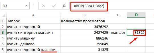

It is not recommended to use nested functions too often, because they are quite difficult to use, errors are possible. And it will take a long time to fix them. 

Function IF can also be used to determine if a particular cell is empty. To achieve this goal, one more function needs to be used − ISBLANK.

Here the syntax is:

=IF(ISBLANK(cell number),”Empty”,”Not empty”).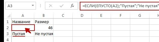

In addition, it is possible to use instead of the function ISBLANK apply the standard formula, but specify that assuming there are no values ​​in the cell.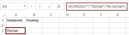

IF – this is one of the most common functions that is very easy to use and it allows you to understand how true certain values ​​are, get results for various criteria, and also determine whether a certain cell is empty.

This function is the foundation for some other formulas. We will now analyze some of them in more detail.

Formula 3: SUMIF

Function SUMMESLI allows you to summarize the data, subject to their compliance with certain criteria.

Syntax

This function, like the previous one, has three arguments. To use it, you need to write such a formula, substituting the necessary values ​​in the appropriate places.

=SUMIF(range, condition, [sum_range])

Let’s understand in more detail what each of the arguments is:

1. Condition. This argument allows you to pass cells to the function, which are further subject to summation.
2. Summation range. This argument is optional and allows you to specify the cells to sum if the condition is false.

So, in this situation, Excel summarized the data on those queries where the number of transitions exceeds 100000.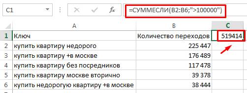

Formula 4: SUMMESLIMN

If there are several conditions, then a related function is used SUMMESLIMN.

Syntax

The formula for this function looks like this:

=SUMIFS(summation_range, condition_range1, condition1, [condition_range2, condition2], …)

The second and third arguments are required, namely “Range of condition 1” and “Range of condition 1”.

Formula 5: COUNTIF and COUNTIFS

This function attempts to determine the number of non-blank cells that match the given conditions within the range entered by the user.

Syntax

To enter this function, you must specify the following formula:

=COUNTIF(range, criteria)

What do the given arguments mean?

1. A range is a set of cells among which the count is to be carried out.
2. Criteria – a condition taken into account when selecting cells.

For example, in this example, the program counted the number of key queries, where the number of clicks in search engines exceeds one hundred thousand. As a result, the formula returned the number 3, which means there are three such keywords.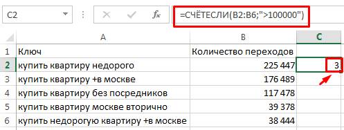

Speaking of related function COUNTIFS, then it, similarly to the previous example, provides the ability to use several criteria at once. Its formula is as follows:

=COUNTIFS(condition_range1, condition1, [condition_range2, condition2],…)

And similarly to the previous case, “Condition Range 1” and “Condition 1” are required arguments, while others can be omitted if there is no such need. The maximum function provides the ability to apply up to 127 ranges along with conditions.

Formula 6: IFERROR

This function returns a user-specified value if an error is encountered while evaluating a formula. If the resulting value is correct, she leaves it.

Syntax

This function has two arguments. The syntax is the following:

=IFERROR(value;value_if_error)

Description of arguments:

1. The value is the formula itself, checked for bugs.
2. The value if error is the result that appears after the error is detected.

If we talk about examples, then this formula will show the text “Error in calculation” if division is impossible.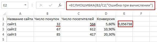

Formula 7: LEFT

This function makes it possible to select the required number of characters from the left of the string.

Its syntax is the following:

=LEFT(text,[num_chars])

Possible arguments:

1. Text – the string from which you want to get a specific fragment.
2. The number of characters is directly the number of characters to be extracted.

So, in this example, you can see how this function is used to see what the titles to the site pages will look like. That is, whether the string will fit in a certain number of characters or not.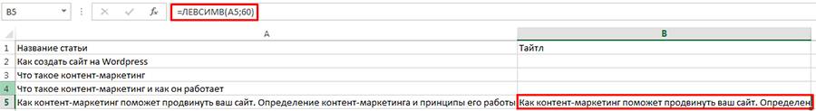

Formula 8: PSTR

This function makes it possible to get the required number of characters from the text, starting with a certain character in the account.

Its syntax is the following:

=MID(text,start_position,number_of_characters).

Argument expansion:

1. Text is a string that contains the required data.
2. The starting position is directly the position of that character, which serves as the beginning for extracting the text.
3. Number of characters – the number of characters that the formula should extract from the text.

In practice, this function can be used, for example, to simplify the names of titles by removing the words that are at the beginning of them.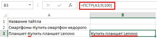

Formula 9: PROPISN

This function capitalizes all letters contained in a particular string. Its syntax is the following:

=REQUIRED(text)

There is only one argument – the text itself, which will be processed. You can use a cell reference.

Formula 10: LOWER

Essentially an inverse function that lowercases every letter of the given text or cell.

Its syntax is similar, there is only one argument containing the text or cell address.

Formula 11: SEARCH

This function makes it possible to find the required element among a range of cells and give its position.

The template for this formula is:

=MATCH(lookup_value, lookup_array, match_type)

The first two arguments are required, the last one is optional.

There are three ways to match:

1. Less than or equal to 1.
2. Exact – 0.
3. The smallest value, equal to or greater than -1.

In this example, we are trying to determine which of the keywords is followed by up to 900 clicks, inclusive.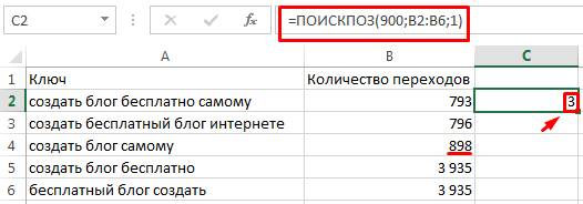

Formula 12: DLSTR

This function makes it possible to determine the length of a given string.

Its syntax is similar to the previous one:

=DLSTR(text)

So, it can be used to determine the length of the article description when SEO-promotion of the site.

It is also good to combine it with the function IF.

Formula 13: CONNECT

This function makes it possible to make several lines from one. Moreover, it is permissible to specify in the arguments both cell addresses and the value itself. The formula makes it possible to write up to 255 elements with a total length of no more than 8192 characters, which is enough for practice.

The syntax is:

=CONCATENATE(text1,text2,text3);

Formula 14: PROPNACH

This function swaps uppercase and lowercase characters.

The syntax is very simple:

=PROPLAN(text)

Formula 15: PRINT

This formula makes it possible to remove all invisible characters (for example, line breaks) from the article.

Its syntax is the following:

=PRINT(text)

As an argument, you can specify the address of the cell.

Conclusions

Of course, these are not all functions that are used in Excel. We wanted to bring some that the average spreadsheet user hasn’t heard of or rarely uses. Statistically, the most commonly used functions are for calculating and deriving an average value. But Excel is more than just a spreadsheet program. In it, you can automate absolutely any function. 

I really hope that it worked out, and you learned a lot of useful things for yourself.