Tables in Microsoft Excel

By itself, an Excel sheet is already one huge table designed to store a wide variety of data. In addition, Microsoft Excel offers an even more advanced tool that converts a range of cells into an “official” table, greatly simplifies working with data, and adds many additional benefits. This lesson will cover the basics of working with spreadsheets in Excel.

When entering data on a worksheet, you may want to format it in a table. Compared to regular formatting, tables can improve the look and feel of a book as a whole, as well as help organize data and simplify its processing. Excel contains several tools and styles to help you quickly and easily create tables. Let’s take a look at them.

The very concept of “table in Excel” can be interpreted in different ways. Many people think that a table is a visually designed range of cells on a sheet, and have never heard of something more functional. The tables discussed in this lesson are sometimes called “smart” tables for their practicality and functionality.

How to make a table in Excel

1. Select the cells you want to convert to a table. In our case, we will select the range of cells A1:D7.
2. On the Advanced tab Home in command group Styles press command Format as a table.
3. Select a table style from the drop-down menu.
4. A dialog box will appear in which Excel refines the range of the future table.
5. If it contains headers, set the option Table with headersthen press OK.
6. The range of cells will be converted to a table in the selected style.

By default, all tables in Excel contain filters, i.e. You can filter or sort data at any time using the arrow buttons in the column headings. For more information about sorting and filtering in Excel, see Working with Data in the Excel 2013 Tutorial.

Changing tables in Excel

By adding a table to a worksheet, you can always change its appearance. Excel contains many tools for customizing tables, including adding rows or columns, changing style, and more.

Adding rows and columns

To add additional data to an Excel table, you need to change its dimension, i.e. add new rows or columns. There are two easy ways to do this:

• Start entering data in an empty row (column) directly adjacent to the table below (on the right). In this case, the row or column will be automatically included in the table.
• Drag the lower right corner of the table to include additional rows or columns.

Style change

1. Select any cell in the table.
2. Then open the tab Constructor and find the command group Table styles. Click on the icon More optionsto see all available styles.
3. Choose the style you want.
4. The style will be applied to the table.

Change settings

You can enable and disable some of the options on the tab Constructorto change the appearance of the table. There are 7 options in total: Header Row, Total Row, Striped Rows, First Column, Last Column, Striped Columns and Filter Button.

1. Select any cell in the table.
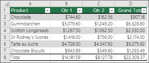
2. On the Advanced tab Constructor in command group Table style options check or uncheck the required options. We will enable the option Total rowto add the total row to the table.
3. The table will change. In our case, a new line appeared at the bottom of the table with a formula that automatically calculates the sum of the values ​​in column D.

These options can change the appearance of the table in different ways, it all depends on its content. You will probably need to experiment a bit with these options to get the look you want.

Deleting a table in Excel

Over time, the need for additional table functionality may disappear. In this case, it is worth deleting the table from the workbook, while retaining all the data and formatting elements.

1. Select any cell in the table and go to the tab Constructor.
2. In a command group Service select team Convert to range.
3. A confirmation dialog box will appear. Click Yes .
4. The table will be converted to a regular range, however, the data and formatting will be preserved.