Selecting a parameter in Excel. “Select parameter” function

The “Select parameter” function in Excel allows you to determine what the initial value was, based on the already known final value. Few people know how this tool works, this article-instruction will help you figure it out.

How the function works

The main task of the “Parameter Selection” function is to help the user of the e-book display the initial data that led to the appearance of the final result. According to the principle of operation, the tool is similar to the “Search for a Solution”, and the “Selection of Material” is considered to be simplified, since even a beginner can handle its use.

Pay attention! The action of the selected function concerns only one cell. Accordingly, when trying to find the initial value for other windows, you will have to carry out all the actions again according to the same principle. Since an Excel function can only operate on a single value, it is considered a limited option.

Features of the function application: a step-by-step overview with an explanation using the example of a product card

To tell you more about how the Parameter Selection works, let’s use Microsoft Excel 2016. If you have a later or earlier version of the application installed, then only some steps may differ slightly, while the principle of operation remains the same.

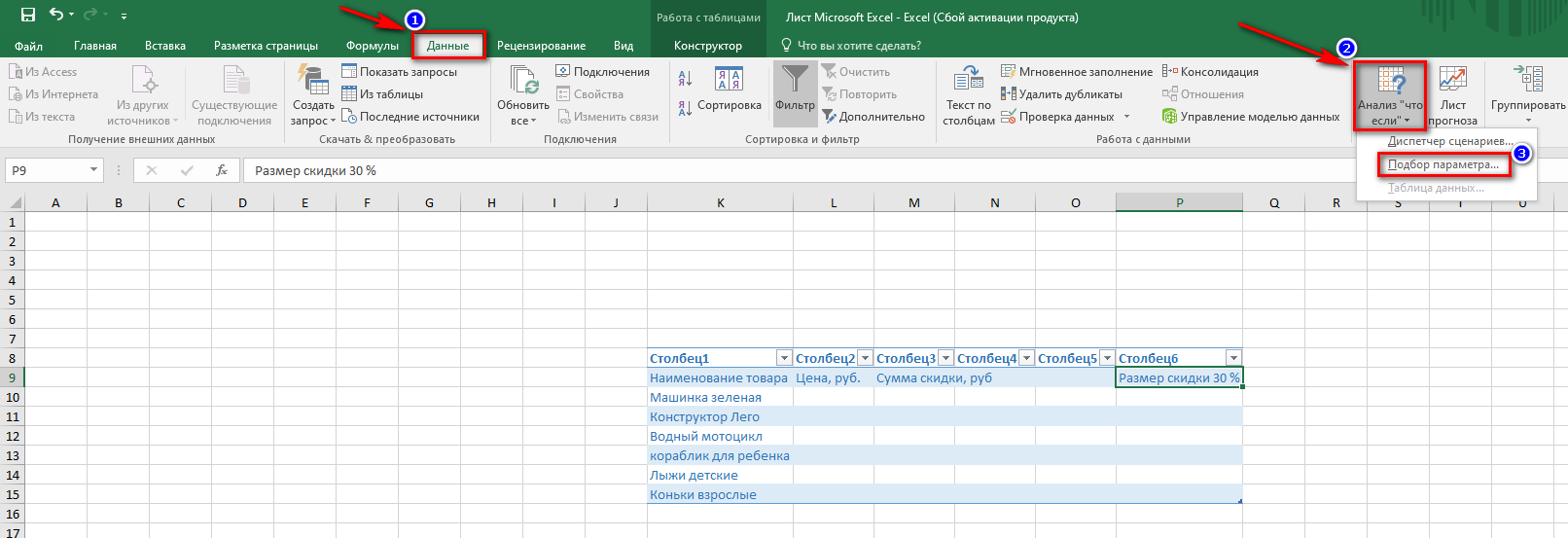
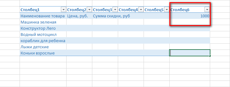
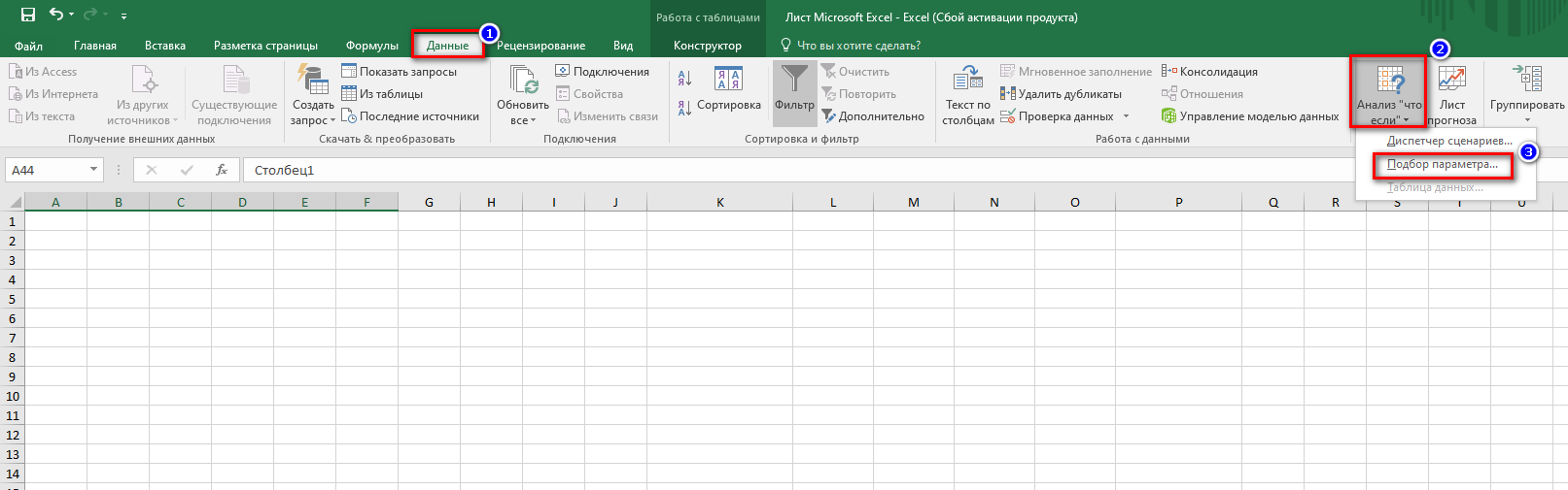
1. We have a table with a list of products, in which only the percentage of the discount is known. We will look for the cost and the resulting amount. To do this, go to the “Data” tab, in the “Forecast” section we find the “Analysis what if” tool, click on the “Parameter selection” function.

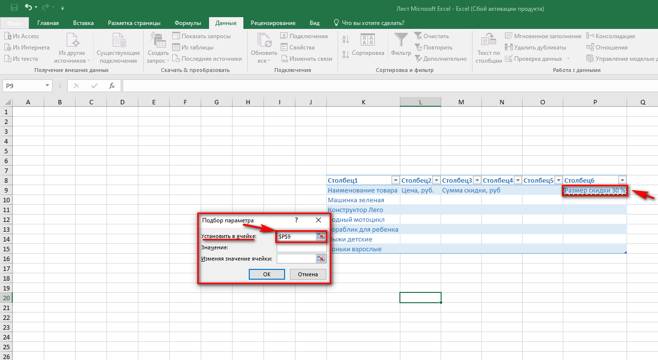
2. When a pop-up window appears, in the “Set in cell” field, enter the desired cell address. In our case, this is the discount amount. In order not to prescribe it for a long time and not periodically change the keyboard layout, we click on the desired cell. The value will automatically appear in the correct field. Opposite the field “Value” indicate the amount of the discount (300 rubles).

Important! The “Select parameter” window does not work without a set value.

3. In the “Change cell value” field, enter the address where we plan to display the initial value of the price for the product. We emphasize that this window should directly participate in the calculation formula. After we make sure that all the values ​​uXNUMXbuXNUMXbare entered correctly, click the “OK” button. To get the initial number, try to use a cell that is in a table, so it will be easier to write a formula.

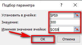
4. As a result, we get the final cost of the goods with the calculation of all discounts. The program automatically calculates the desired value and displays it in a pop-up window. In addition, the values ​​are duplicated in the table, namely in the cell that was selected to perform the calculations.

On a note! Fitting calculations to unknown data can be performed using the “Select parameter” function, even if the primary value is in the form of a decimal fraction.

Solving the equation using the selection of parameters

For example, we will use a simple equation without powers and roots, so that we can visually see how the solution is made.

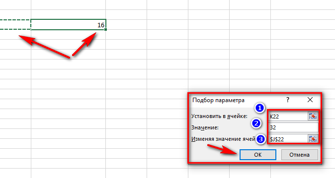
1. We have an equation: x+16=32. It is necessary to understand what number is hidden behind the unknown “x”. Accordingly, we will find it using the “Parameter Selection” function. To begin with, we prescribe our equation in the cell, after putting the “=” sign. And instead of “x” we set the address of the cell in which the unknown will appear. At the end of the entered formula, do not put an equal sign, otherwise we will display “FALSE” in the cell.

2. Let’s start the function. To do this, we act in the same way as in the previous method: in the “Data” tab we find the “Forecast” block. Here we click on the “Analyze what if” function, and then go to the “Select parameter” tool.

3. In the window that appears, in the “Set value” field, write the address of the cell in which we have the equation. That is, this is the “K22” window. In the “Value” field, in turn, we write the number that equals the equation – 32. In the “Changing the value of the cell” field, enter the address where the unknown will fit. Confirm your action by clicking on the “OK” button.

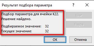
4. After clicking on the “OK” button, a new window will appear, in which it is clearly stated that the value for the given example was found. It looks like this:

In all cases when the calculation of unknowns is performed by “Selection of parameters”, a formula should be established; without it, it is impossible to find a numerical value.

Advice! However, using the “Parameter selection” function in Microsoft Excel in relation to equations is irrational, since it is faster to solve simple expressions with an unknown on your own, and not by searching for the right tool in an e-book.

To summarize

In the article, we analyzed for the use case of the “Parameter selection” function. But note that in the case of finding the unknown, you can use the tool provided that there is only one unknown. In the case of tables, it will be necessary to select parameters individually for each cell, since the option is not adapted to work with a whole range of data.