INDEX function in Excel. How to work with the INDEX function in Excel, and how it can be useful

The spreadsheet processor has an extensive number of functions that allow the user to carry out various types of information processing. The INDEX function helps to implement the search for values ​​in the designated location of the specified range, and then displays the result in the selected sector. This article will detail how to use the INDEX function in a variety of ways.

Description of the INDEX function

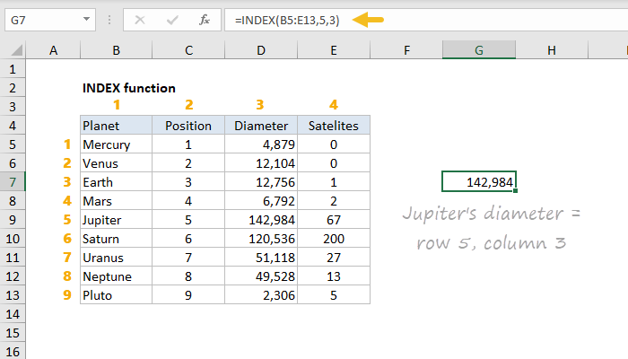
INDEX is a function integrated into a spreadsheet that allows you to get information from a table, provided that the user knows the line and column number in which this information is located.

What the function returns

This function returns values ​​from a specific row and column of a table.

Syntax

There are four syntax variations for this function. Two versions:

1. =INDEX(array; row_number; [column_number]).
2. =INDEX(reference; line_number; [column_number], [area_number]).

Two English versions:

1. =INDEX (array, row_num, [col_num]).
2. =INDEX (array, row_num, [col_num], [area_num]).

Function arguments

Let’s take a closer look at what each of the arguments below means:

• array – indicates a range of sectors or an array of data to be searched;
• row_num – indicates the number of the line where the required values ​​uXNUMXbuXNUMXbare located;
• [col_num] – indicates the number of the column where the required values ​​are located. This parameter is optional. In the case when the line number argument is not described in the INDEX function, this parameter must be specified;
• [area_num] – used when the array has a certain number of ranges. The parameter is optional and is used to select absolutely all ranges.

Additional Information

Consider some features of the function that you need to know when using it:

• When the column or row number is zero, the function will return the data of the entire column or row.
• If you use the INDEX function before a cell reference, the cell reference will be returned instead of the value. We will talk about this in more detail in the examples below.
• Typically, the INDEX function is used in conjunction with the MATCH function.
• The INDEX function differs from the VLOOKUP function in that it returns data both to the left of the desired measure and to the right.
• INDEX can be used in 2 different forms: “Data Links” and “Data Array”.
• “Array” is used in cases where it is necessary to find indicators based on certain numbers of columns and rows of tabular information.
• “Data links” are used when it is necessary to find indicators in a number of tables in order to select a plate, and then help the function to search by column and row number.

How does the INDEX function work in Excel?

Let’s consider the work process of the INDEX function with different data types in a spreadsheet.

INDEX function in Excel step by step instructions

The step-by-step instruction for working with the INDEX function has a different form depending on what it is used for. It can be used to work with arrays, references, and other auxiliary operators.

INDEX function for arrays

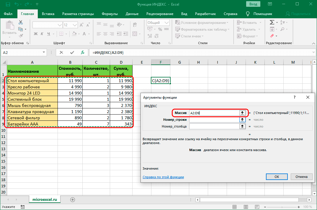
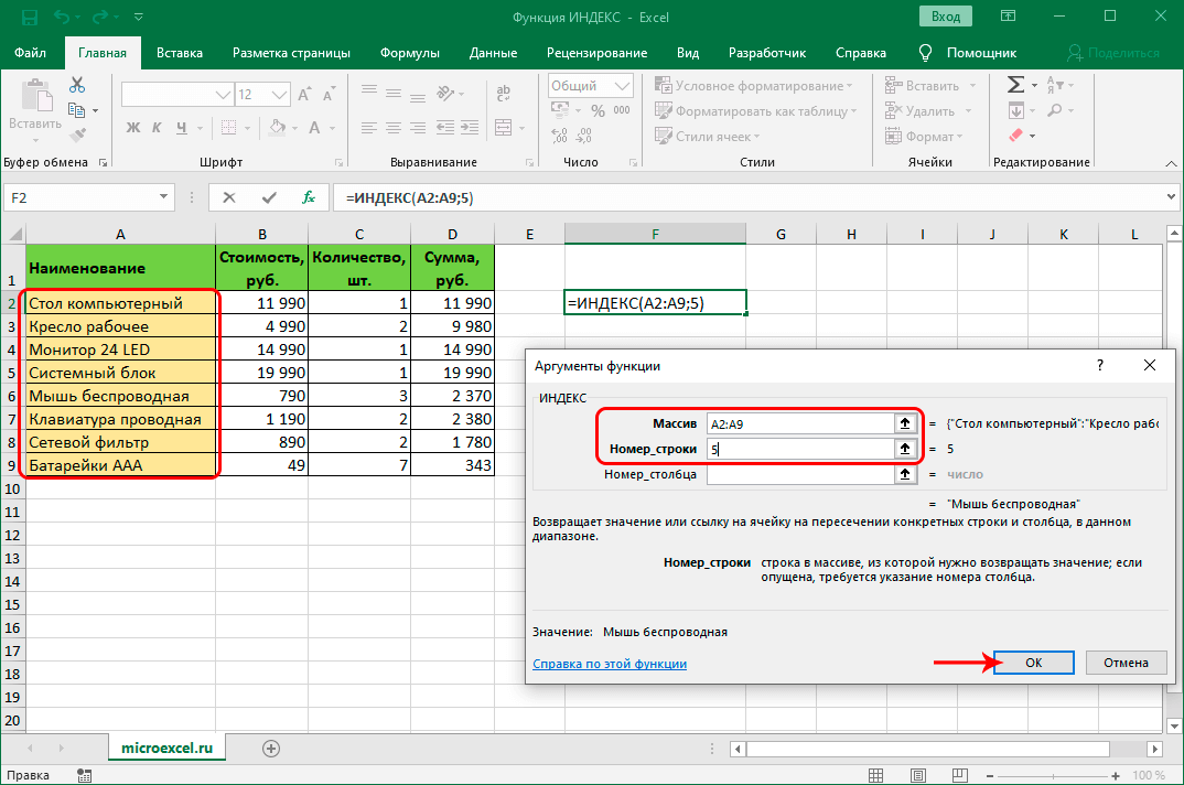
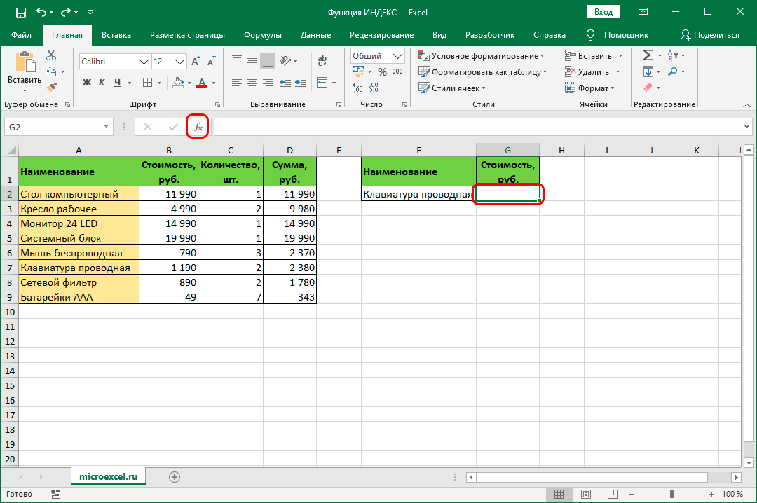
For example, there is a plate with the names of products, their cost, number and final amount.

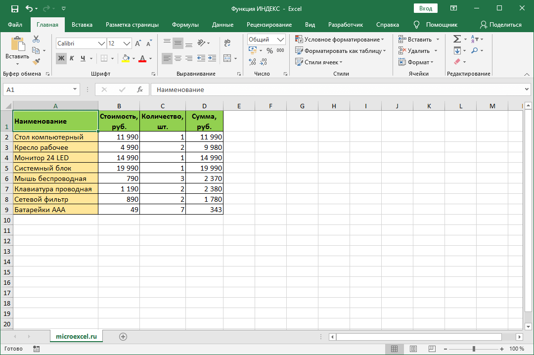
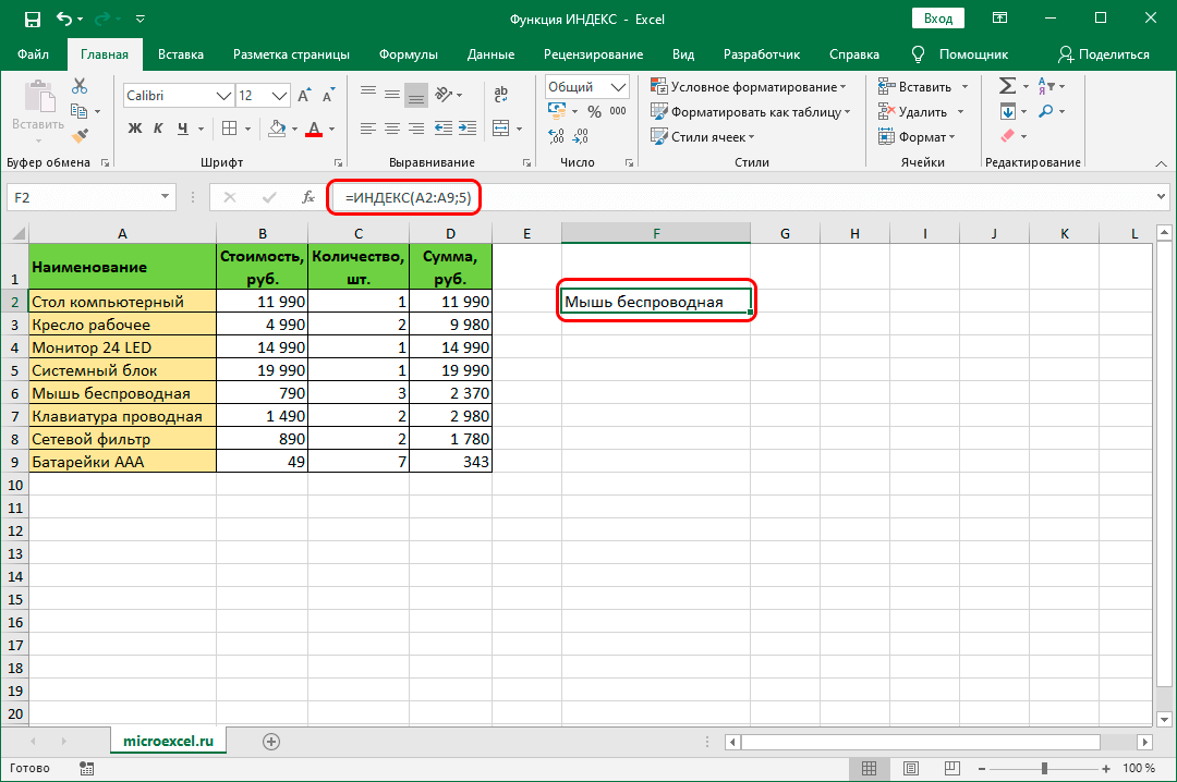
Purpose: in the selected sector, show the name of the fifth position in the list. The step by step guide looks like this:

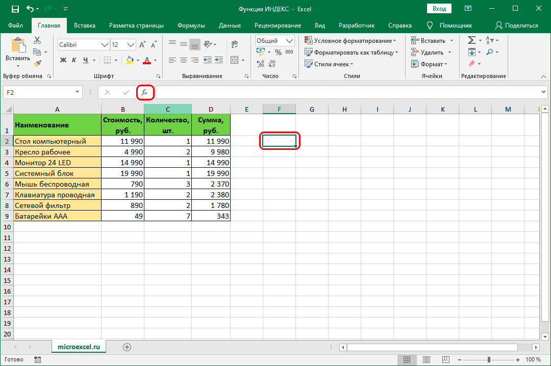
1. We click on the sector in which we want to display the result of manipulations in the future. We click the “Insert Function” button located next to the line for entering formulas.

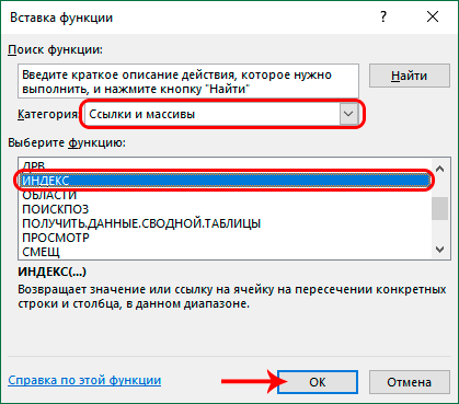
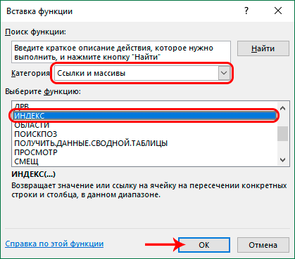
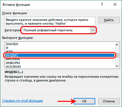
2. A window called “Insert function” opens on the display. Expand the list located next to the inscription “Category:”, and click “Links and arrays”. Next, in the window with a list of functions, select “INDEX”. After completing all the steps, click on the “OK” button.

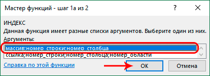
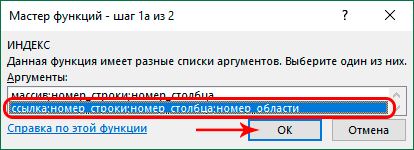
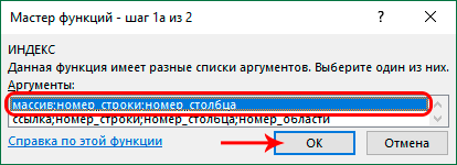
3. A small window appeared on the screen prompting you to select a set of arguments. Select the 1st suggested option and click OK.

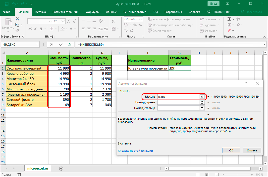
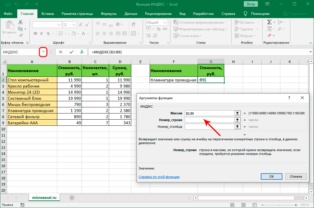
4. In the next window, you must specify the arguments. In the “Array” field, enter the range within which the function will work. Coordinates can be entered independently or by selecting the required area on the worksheet with the help of a clamped LMB.

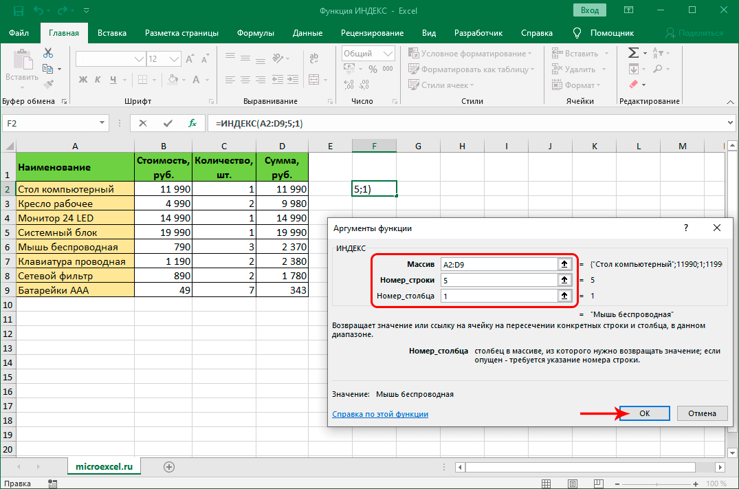
5. In the field “Line_number” we drive in the number 5, since this is required by the task set before us.
6. In the “Column_number” field, we drive in the number 1, since the names of the values ​​u1buXNUMXbare located in the XNUMXst column of the array.
7. After making all the settings, click “OK”.

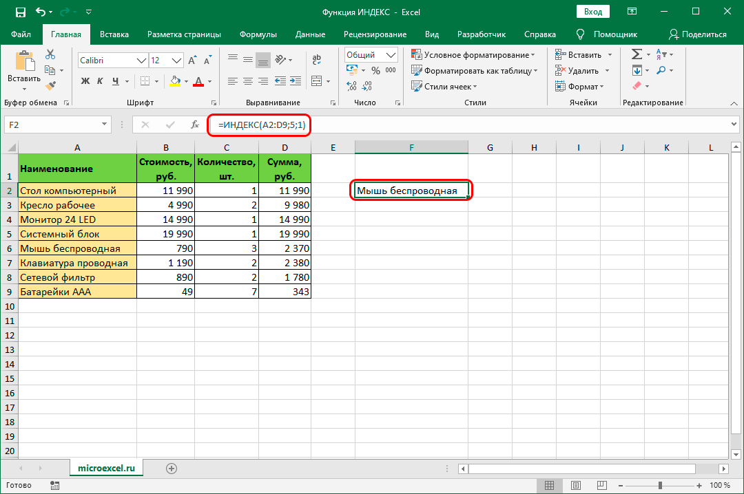
8. The final result appeared in the selected sector.

Pay attention! One of the arguments can be omitted if the array is one-dimensional.

Such actions look like this:

1. In the “Array” line, it is necessary to select only the cells of the first column. We enter the row number – 5, and do not fill in the column number, because the array is one-dimensional.

2. We click on “OK”. As a result, in the selected sector we obtain a similar result.

INDEX function for links

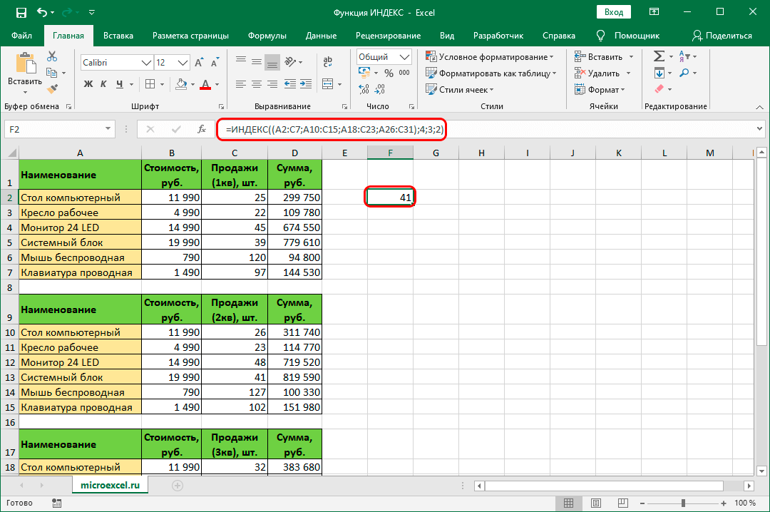
The INDEX function can work with a number of tables at once. To implement this action, you need a list of values ​​for links with the “Region_Number” field. For example, we have four tables. They contain data on sales for a different period of time.

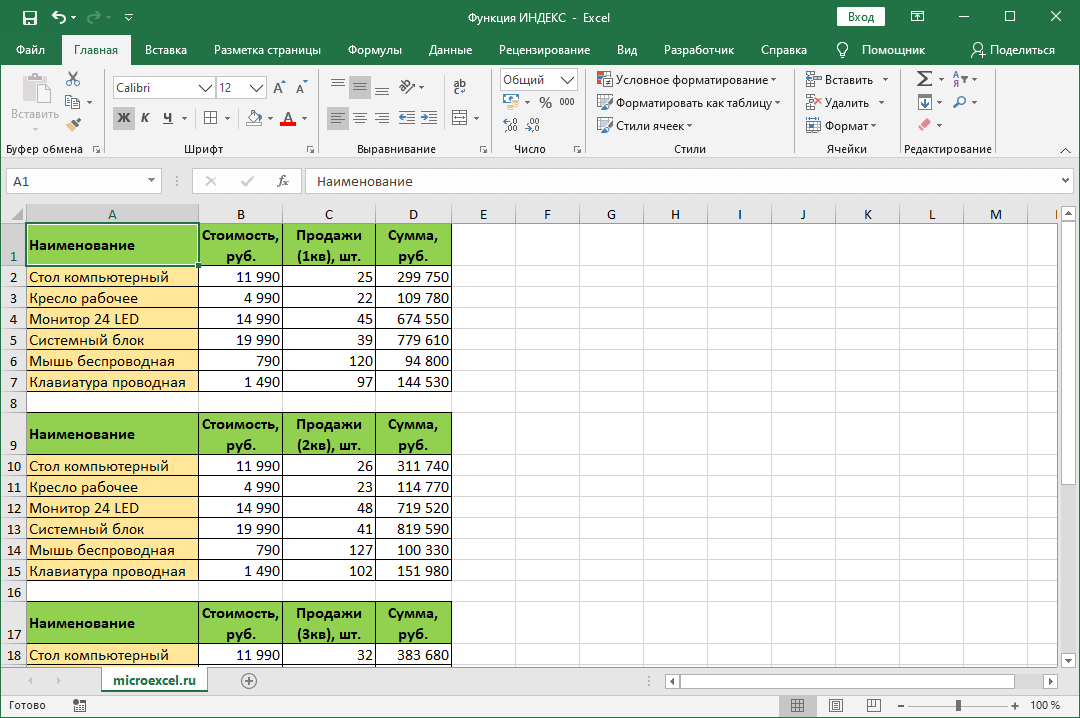
Purpose: to identify the number of sales in the 4th position for the 2nd quarter in pieces. The walkthrough looks like this:

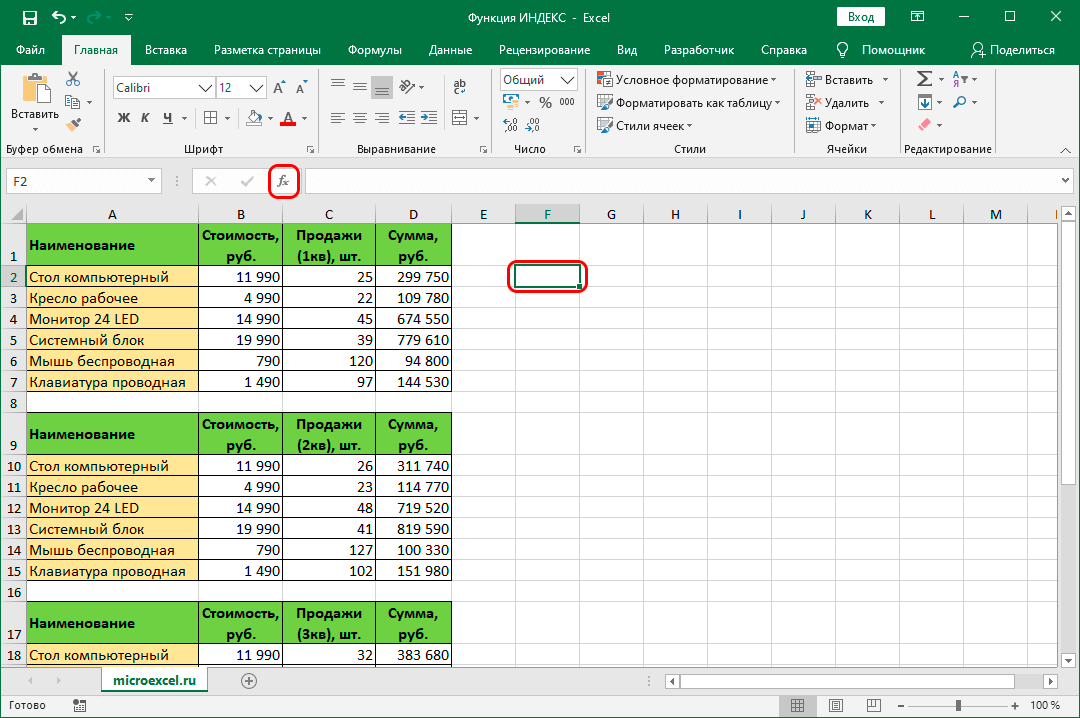
1. We click on the sector in which we want to display the result of manipulations in the future. We click the “Insert Function” button located next to the line for entering formulas.

2. A window titled “Insert Function” opens on the display. Expand the list located next to the inscription “Category:”, and click “Links and arrays”. Next, in the window with a list of functions, select “INDEX”. After completing all the steps, click “OK”.

3. A small window appeared on the screen prompting you to select a set of arguments. Select the second suggested option and click OK.

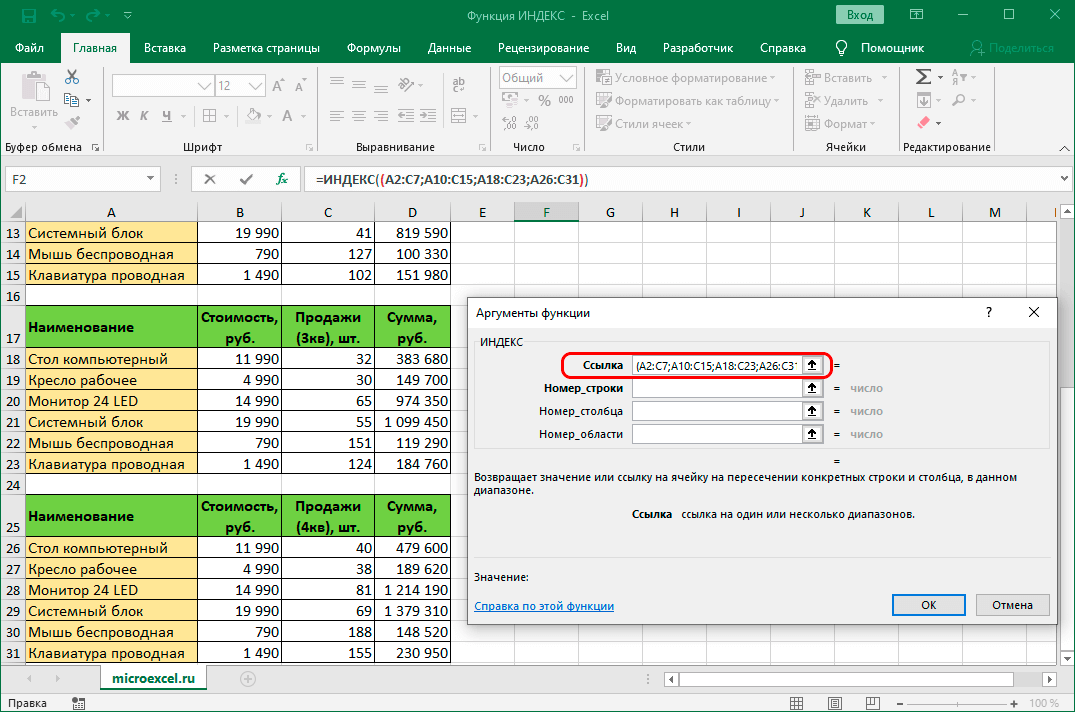
4. In the next window, you must specify the arguments. In the “Reference” field, enter the same values ​​that were entered in the “Array” field in the previous example. The main difference is that we specify not one range, but four at once, separating them with a “;” sign. After the description, put “(” at the beginning and “)” at the end.

5. In the “Line_number” field, enter the value 4, according to the condition of our task.
6. In the line “Column_number” we enter the value 3, because we need to find out the number of sales in pieces.
7. In the line “Region number” we enter the value 2, because according to the condition of the problem, we need to find out information on the second quarter.

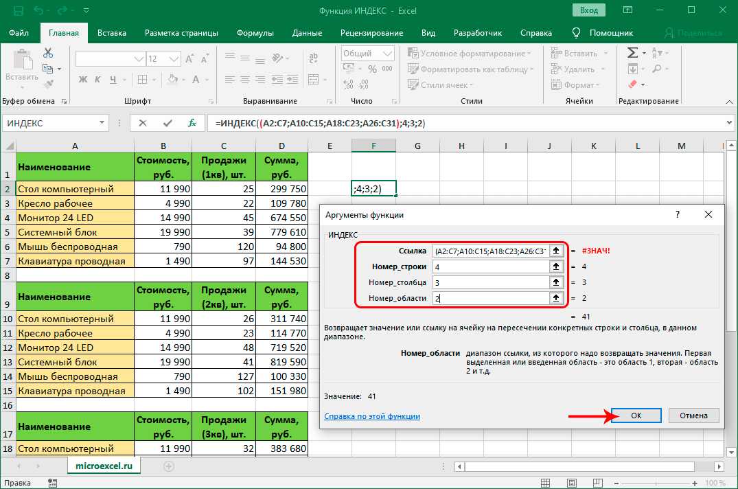
8. After carrying out all the manipulations, click on the “OK” button. Done, the selected sector has the answer we need.

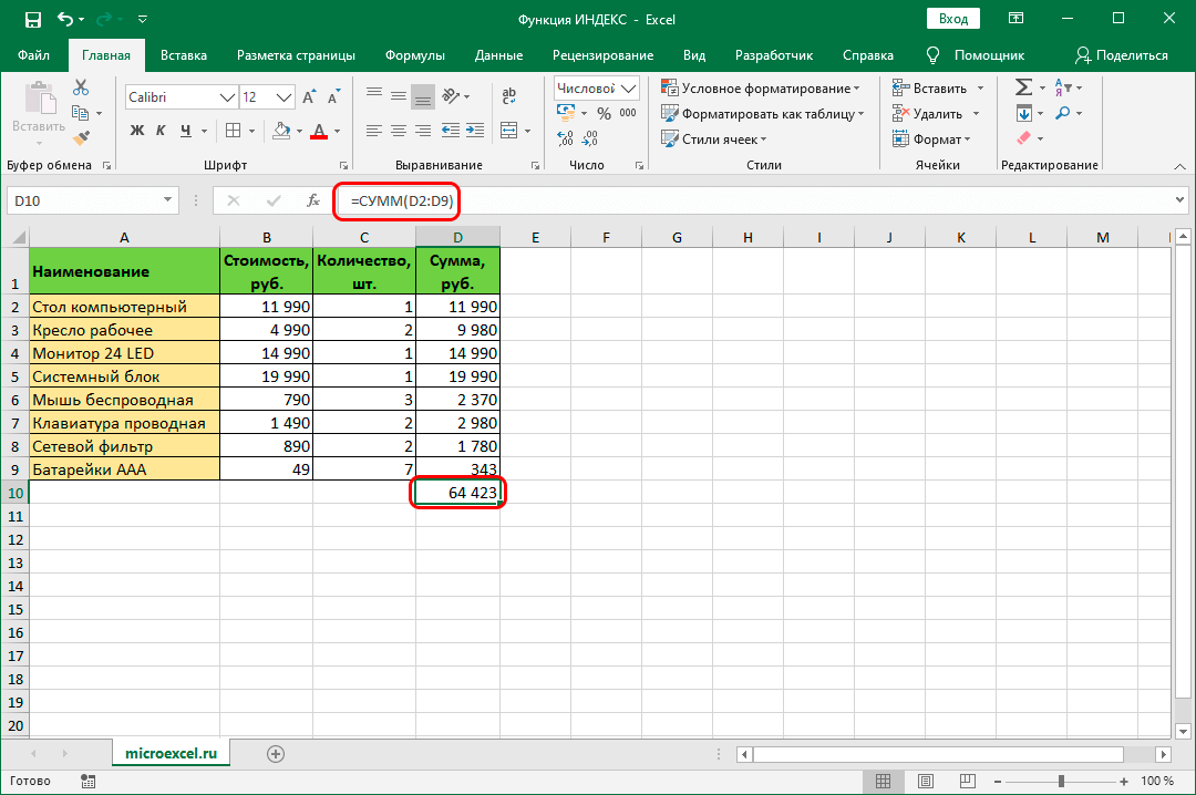
Use with the SUM operator

The INDEX function is often used in conjunction with the SUM operator. General view of the operator: =SUM(Array_address). By applying the SUM to the table we are considering, we can get the final amount. The formula for calculating the amount will look like this: =SUM(D2:D9).

You can slightly edit the formula by embedding the INDEX function in it. The walkthrough looks like this:

1. For the first argument of the SUM operator, we set the coordinates of the sector that is the start point of the summing range.
2. The 2nd argument is set using the INDEX function. Click on the line to enter formulas and drive in the following value: =SUM(D2:INDEX(D2:D9)). The number 8 indicates that we are setting a limit for the selected range between sectors D2 and D9.

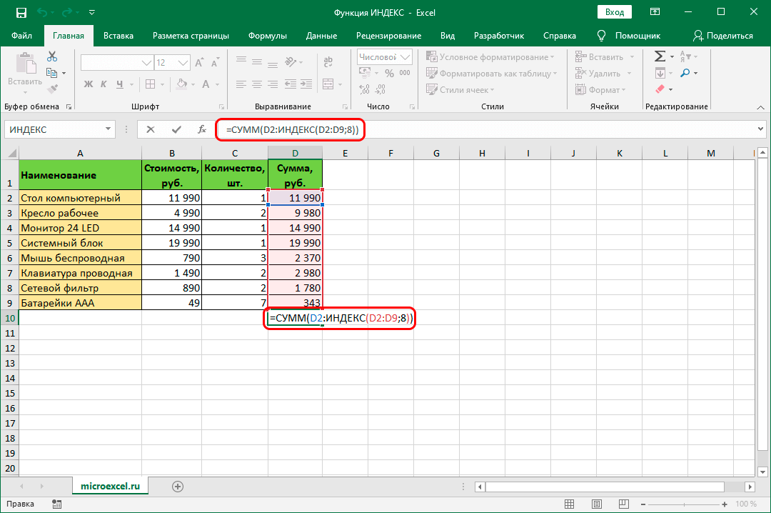
3. Press the “Enter” key to display the final result in the initially selected sector.

Combination with MATCH function

We turn to the analysis of more complex problems. Below is an example of using the INDEX function with the MATCH operator. MATCH allows you to return the specified indicator in the selected range of sectors. General view of the formula: =MATCH(Lookup_Value, Lookup_Array, [Match_Type]). Let’s analyze each function indicator in more detail:

• The desired value. This argument specifies the value to look for in the selection.
• The array being viewed. Area of ​​sectors to search for the desired indicator.
• Mapping type. The argument is optional and is used to refine your search.

For clarity, the use of two functions will analyze everything on specific examples. Let’s take the same table that we considered in the previous examples. There is a small plate next to it, in which there is one empty value for the name and price. Purpose: using MATCH and INDEX, to add to sector G2 a function that displays a certain value depending on the name specified in the sector. The walkthrough looks like this:

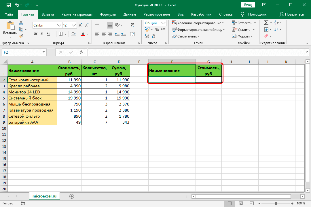
1. First, fill in cell F1.

2. We click on the sector in which we want to display the result of manipulations in the future. We click the “Insert Function” button located next to the line for entering formulas.

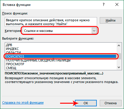
3. A window titled “Insert Function” opens on the display. Expand the list located next to the inscription “Category:”, and click “Links and arrays”. Next, in the window with a list of functions, select “INDEX”. After completing all the steps, click on “OK”.

4. A small window appeared on the screen prompting you to select a set of arguments. Select the first suggested option and click OK.

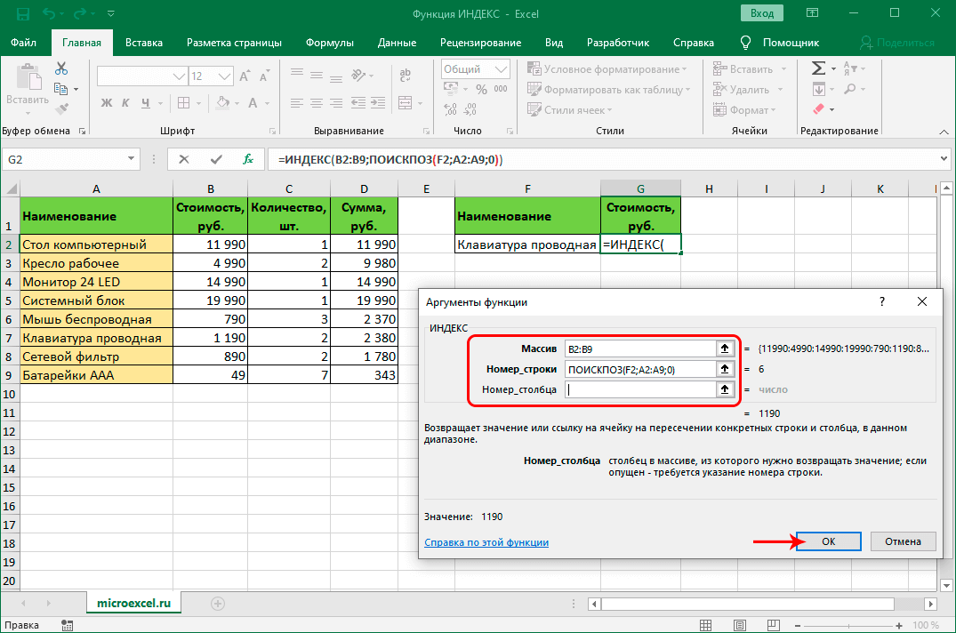
5. In the “Array” line, enter the sector of the column in which the cost of the positions is located.

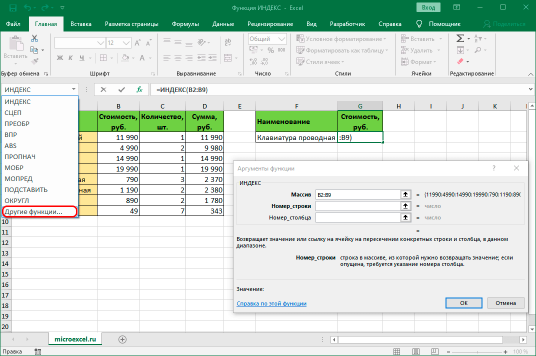
6. In the line “Line_number” add the MATCH function. To implement this action, click on the small arrow located near the “Insert function” element. A drop-down list will open, where you need to select “Other functions”. A new window “Function Wizard” appeared, in which we click “References and Arrays”, and then select MATCH. After carrying out all the manipulations, click “OK”.

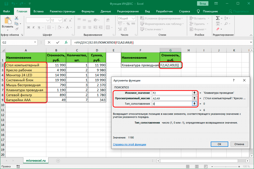
7. In the “Lookup_value” field, enter the coordinates of the cell, according to the content of which the search will be carried out in the main array. In the “Viewed_array” field, we drive in the range to search for the desired indicator. Enter 0 in the Match_Type field.

8. In the line for entering formulas, click on “INDEX”.

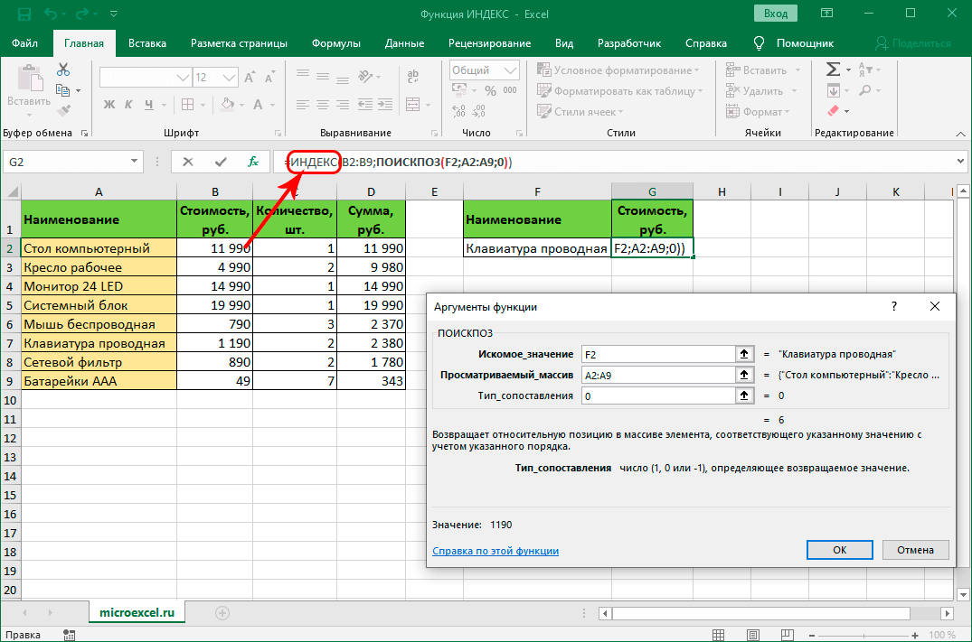
9. The list of arguments is displayed again on the screen. We notice that the indicators are automatically filled with the necessary data. Do not touch anything and click on “OK”. It is worth noting that the “Line_Number” field can be filled in independently using the syntax of the MATCH operator.

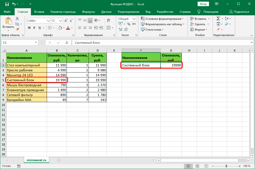
10. As a result, we got the necessary result in the selected sector – the value of the position. Various cost changes in the main table will be reflected in this cell. The same rule applies to changing the name in the auxiliary plate.

Handling multiple tables

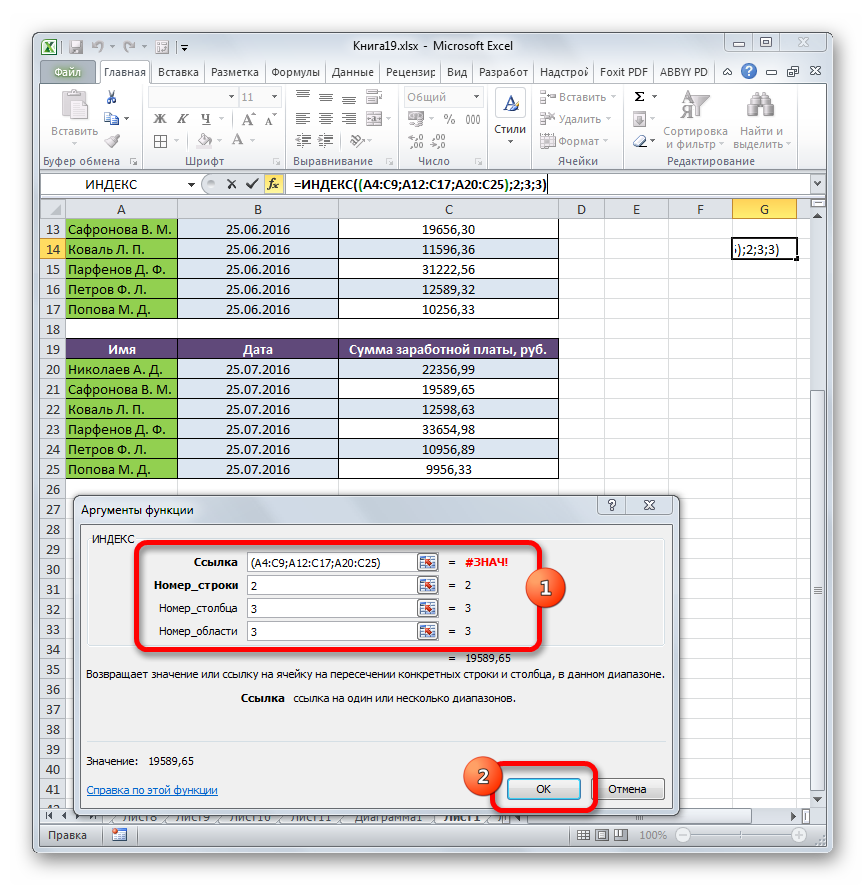
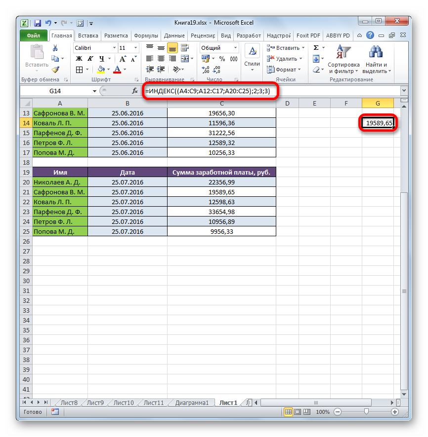
Consider the process of processing multiple tables. For example, we have 3 tables. They display the salary of employees by month. Purpose: to reveal the salary of the second employee for the 3rd month. The walkthrough looks like this:

1. We click on the cell in which we want to display the result of manipulations in the future. We click the “Insert Function” button located next to the line for entering formulas.
2. A window called “Insert function” opens on the display. Expand the list next to “Category:” and click “Links and Arrays”. Next, in the window with a list of functions, select “INDEX”. After completing all the steps, click on the “OK” button.
3. A small window appeared on the screen prompting you to select a set of arguments. Select the 2st suggested option and click OK.
4. In the line “Link” enter the coordinates of each range. In the line “Line number” we drive in the number 2, because we are searching for the 2nd surname in the list. In the line “Column number” we enter the number 3. In the line “Area number” we also drive in the number 3. After all the manipulations, click on “OK”.

5. The required results were displayed in the pre-selected sector.

Examples of using the INDEX function in Excel

Let’s take a look at another usage example. For example, we have the following table information:

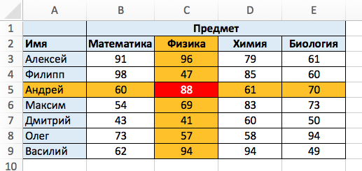
To find out the result of Andrey in the discipline “Physics”, you must apply the following formula: =INDEX($B$3:$E$9). Here we have determined the indicators of the desired range: $B$3:$E$9. The number 3 means the number of the line where Andrey’s result is located. The number 2 means the number of the column where the discipline “Physics” is located.

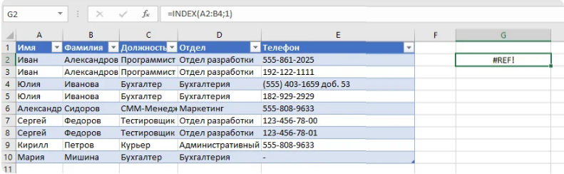
Errors

The INDEX function throws an error if one of the arguments is out of range.

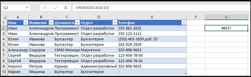
An error occurs if the spreadsheet does not understand which sector to return.

Conclusion

The INDEX function is an efficient operator in the Excel spreadsheet that allows you to implement a huge list of various actions. Having studied the work with this operator, you can significantly speed up the process of working with large amounts of information.