AutoFilter function in Excel. Application and setting

When you need to find one or more rows in a large table, you have to spend a lot of time scrolling through the sheet and looking for the right cells with your eyes. The built-in Microsoft Excel filter makes it easy to find data among many cells. Let’s find out how to enable and disable the automatic filter, and analyze the possibilities that it gives users.

How to enable AutoFilter in Excel

There are several ways to get started using this option. Let’s analyze each of them clearly. The result of turning on the filter will be the appearance of a square button with an arrow next to each cell in the table header.

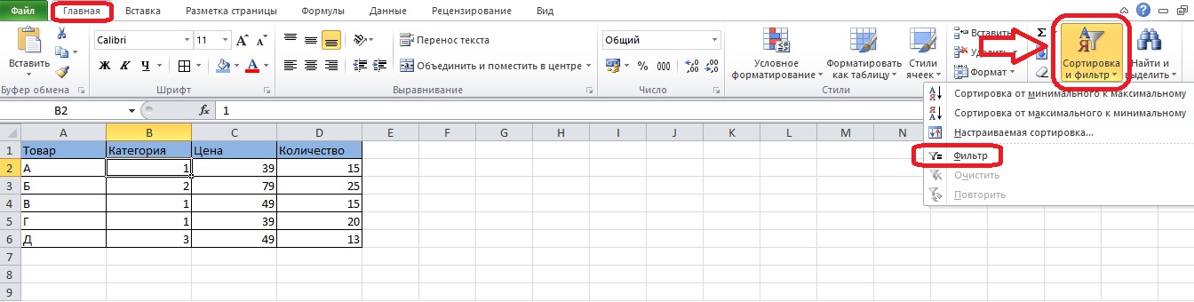
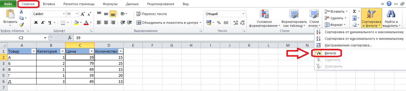
1. The Home tab contains several sections. Among them – “Editing”, and you need to pay attention to it.
2. Select the cell for which the filter will be set, then click on the “Sort and Filter” button in this section.
3. A small menu will open where you need to select the “Filter” item.

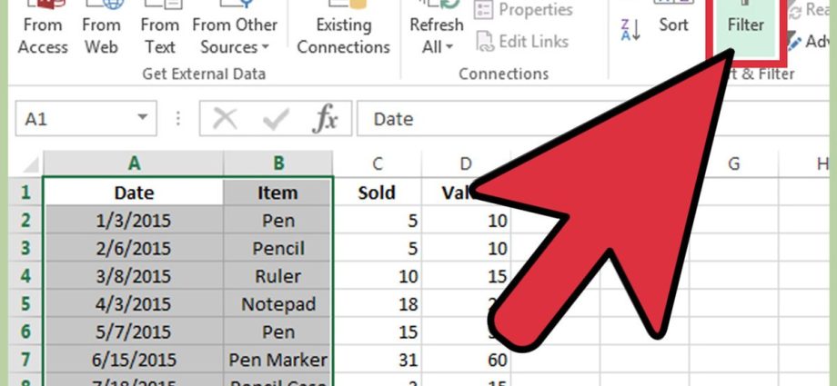
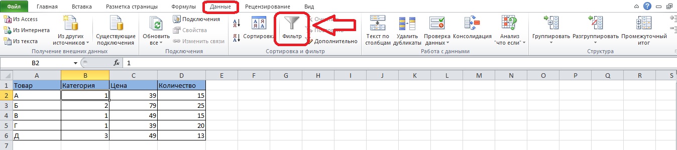
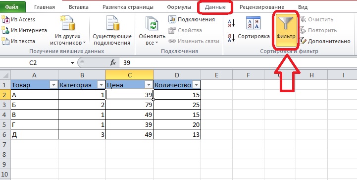
1. The second method requires another tab in the Microsoft Excel menu – it is called “Data”. It has a separate section reserved for sorting and filters.
2. Again, click on the desired cell, open “Data” and click on the “Filter” button with the image of a funnel.

Important! You can only use a filter if the table has a header. Setting the filter on a table without headings will result in the loss of data in the top row – they will disappear from view.

Setting up a filter by table data

The filter is often used in large tables. It is needed in order to quickly view the lines of one category, temporarily separate them from other information.

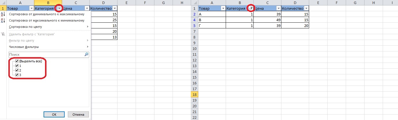
1. You can only filter data by column data. Open the menu by clicking on the arrow in the header of the selected column. A list of options will appear with which to sort the data.
2. To begin with, let’s try the simplest thing – remove a few checkmarks, leaving only one.
3. As a result, the table will consist only of rows containing the selected value.
4. A funnel icon will appear next to the arrow, indicating that the filter is enabled.

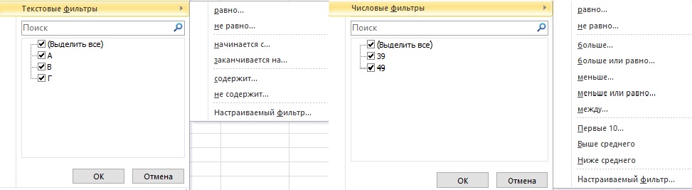
Sorting is also carried out by text or numeric filters. The program will leave lines on the sheet that meet the established requirements. For example, the text filter “equal to” separates the rows of the table with the specified word, “not equal” works the other way around – if you specify a word in the settings, there will be no rows with it. There are text filters based on initial or ending letter.

Numbers can be sorted by filters “greater than or equal”, “less than or equal”, “between”. The program is able to highlight the first 10 numbers, select data above or below the average value. Full list of filters for text and numeric information:

If the cells are shaded and a color code is set, the ability to sort by color opens. Cells of the selected color move to the top. The filter by color allows you to leave on the screen rows whose cells are colored in the shade selected from the list.

Important! Separately, it is worth noting the “Advanced …” function in the “Sort and Filter” section. It is designed to expand the filtering capabilities. Using the advanced filter, you can set the conditions manually as a function.

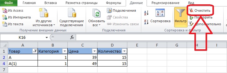
The filter action is reset in two ways. The easiest way is to use the “Undo” function or press the key combination “Ctrl + Z”. Another way is to open the data tab, find the “Sort and Filter” section and click the “Clear” button.

Custom Filter: Customize by Criteria

Data filtering in the table can be configured in a way that is convenient for a particular user. To do this, the “Custom filter” option is enabled in the autofilter menu. Let’s figure out how it is useful and how it differs from the filtering modes specified by the system.

1. Open the sort menu for one of the columns and select the “Custom Filter…” component from the text/number filter menu.
2. The settings window will open. On the left is the filter selection field, on the right is the data on the basis of which sorting will work. You can filter by two criteria at once – that’s why there are two pairs of fields in the window.

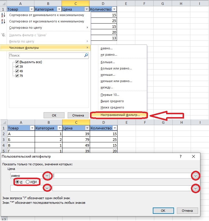
3. For example, let’s select the “equals” filter on both rows and set different values ​​- for example, 39 on one row and 79 on the other.
4. The list of values ​​is in the list that opens after clicking on the arrow, and corresponds to the contents of the column where the filter menu was opened. You need to change the choice of fulfilling the conditions from “and” to “or” so that the filter works, and does not remove all the rows of the table.
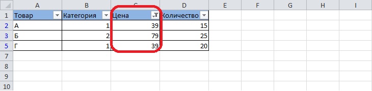
5. After clicking the “OK” button, the table will take on a new look. There are only those lines where the price is set to 39 or 79. The result looks like this:

Let’s observe the work of text filters:

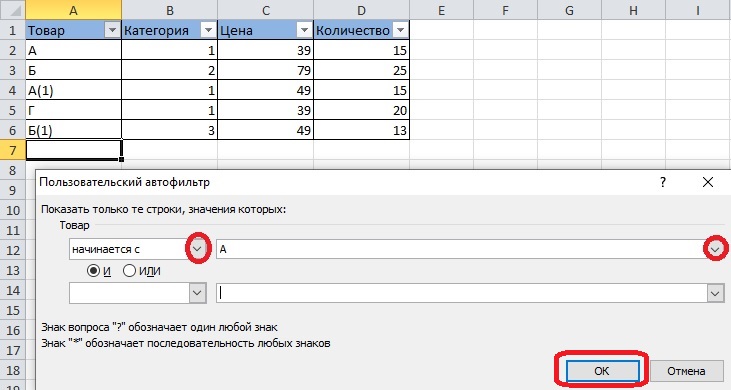
1. To do this, open the filter menu in the column with text data and select any type of filter – for example, “starts with …”.
2. The example uses one autofilter line, but you can use two.

Select a value and click on the “OK” button.

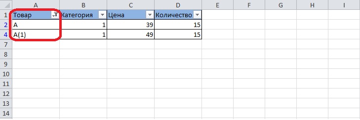
3. As a result, two lines starting with the selected letter remain on the screen.

Disabling AutoFilter via the Excel Menu

To turn off the filter on the table, you need to turn to the menu with tools again. There are two ways to do this.

1. Let’s open the “Data” tab, in the center of the menu there is a large “Filter” button, which is part of the “Sort and Filter” section.
2. If you click this button, the arrow icons will disappear from the header, and it will be impossible to sort the rows. You can turn filters back on if needed.

Another way does not require moving through the tabs – the desired tool is located on the “Home”. Open the “Sort and Filter” section on the right and click on the “Filter” item again.

Advice! To determine whether sorting is on or off, you can look not only at the table header, but also at the menu. The “Filter” item is highlighted in orange when it is turned on.

Conclusion

If the autofilter is configured correctly, it will help you find information in a table with a header. Filters work with numeric and textual data, which helps the user to greatly simplify the work with the Excel spreadsheet.