How to Subtract Numbers in Excel – 5 Practical Examples

The Microsoft Excel spreadsheet service is often used to organize data in numerical format and perform calculations on it. Subtraction is one of the basic mathematical operations, not a single complex calculation can do without it. There are several ways to embed subtractive cells in a table, each of which will be discussed in detail below.

How to make a subtraction function in excel

Subtraction in the table is the same as on paper. The expression must consist of a minuend, a subtrahend, and a “-” sign between them. You can enter the minuend and subtrahend manually or select cells with this data.

Pay attention! There is one condition that distinguishes subtraction in Excel from a normal operation. Every function in this program starts with an equal sign. If you do not put this sign before the composed expression, the result will not appear in the cell automatically. The program will perceive what is written as text. For this reason, it is important to always put the “=” sign at the beginning.

It is necessary to make a formula with the “-” sign, check the correctness of the choice of cells or the entry of numbers and press “Enter”. In the cell where the formula was written, the difference of two or more numbers will immediately appear. Unfortunately, there is no ready-made subtraction formula in the Function Manager, so you have to go other ways. Using the catalog of formulas will only work for more complex calculations, for example, those that use complex numbers. Let’s look at all the working methods below.

subtraction procedure

First, as mentioned, you need to write an equal sign in the term of the functions or in the cell itself. This shows that the value of the cell is equal to the result of the math operation. Further, in the expression, a reduced one should appear – a number that will become less as a result of the calculation. The second number is subtracted, the first one becomes less by it. A minus is placed between the numbers. You don’t need to make a dash from a hyphen, otherwise the action won’t work. Let’s explore five ways to subtract in Excel spreadsheets. Each user will be able to choose a convenient method for themselves from this list.

Example 1: Difference of Specific Numbers

The table is drawn up, the cells are filled, but now you need to subtract one indicator from another. Let’s try to subtract one known number from another.

1. First you need to select the cell in which the result of the calculation will be. If there is a table on the sheet, and it has a column for such values, you should stop at one of the cells in this column. In the example, we will consider subtraction in a random cell.
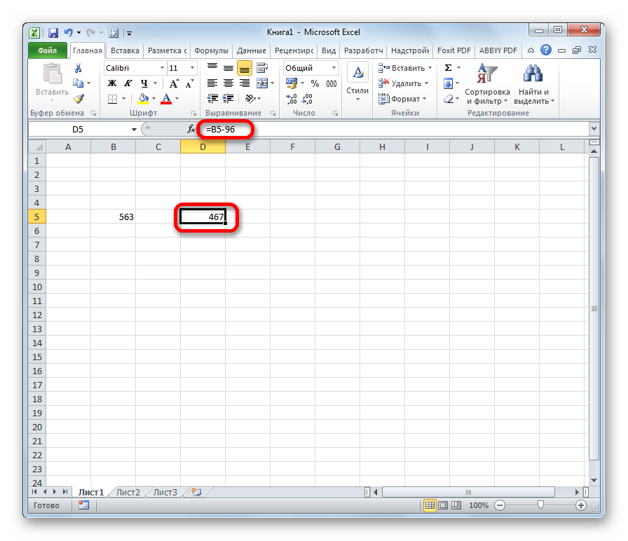
2. Double click on it so that a field appears inside. In this field, you need to enter an expression in the form that was described earlier: the “=” sign, reduced, minus sign and subtracted. You can also write an expression in the function line, which is located above the sheet. The result of all these actions looks like this:

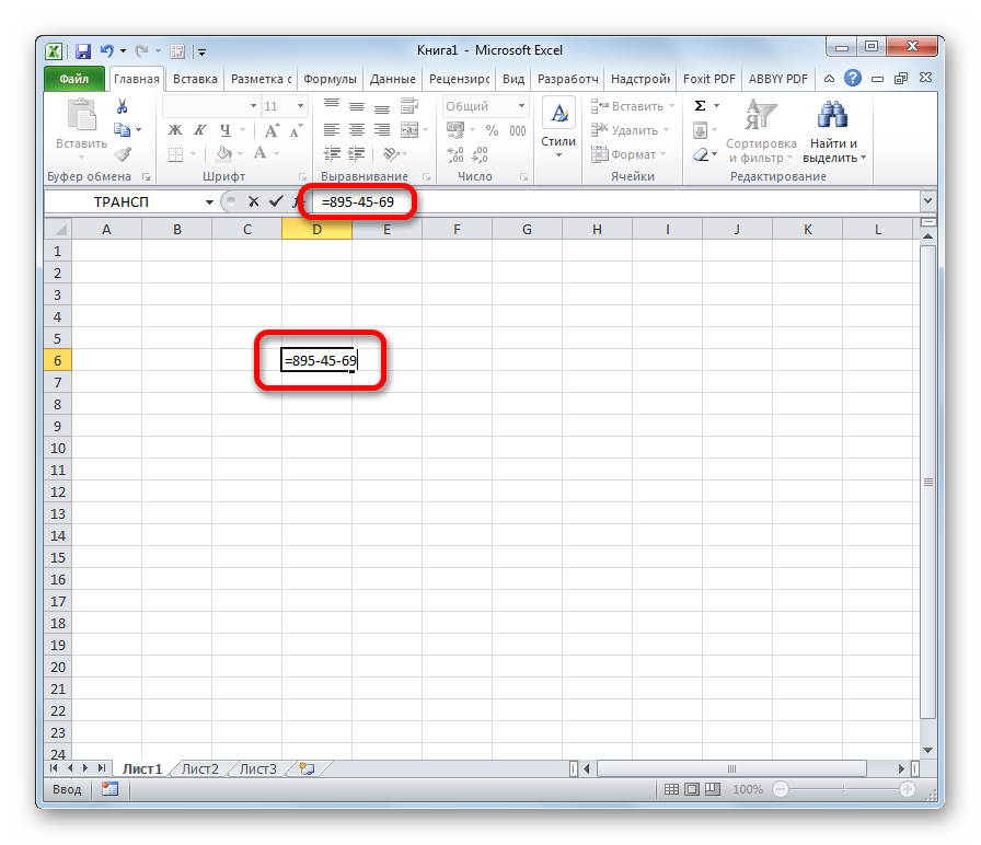
Pay attention! There can be any number of subtrahends, it depends on the purpose of the calculation. Before each of them, a minus is required, otherwise the calculations will not be carried out correctly.

3. If the numbers in the expression and its other parts are written correctly, you should press the “Enter” key on the keyboard. The difference will immediately appear in the selected cell, and in the function line you can view the written expression and check it for errors. After performing automatic calculations, the screen looks like this:

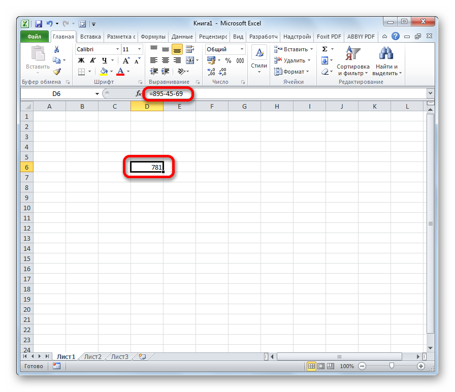
The spreadsheet Microsoft Excel is also designed for convenient calculations, so it works with positive and negative numbers. It is not necessary that the minuend be a larger number, but then the result will be less than zero.

Example 2: subtracting a number from a cell

Working with table cells is the main task of Excel, so you can perform a variety of actions with them. For example, you can compose a mathematical expression where a cell is reduced and a number is subtracted, or vice versa.

1. The first action is to select the cell for the formula again and put an equal sign in it.
2. Next, you need to act differently than in the first method – you need to find a cell in the table with a value that will decrease as a result of subtraction, and click on it. A mobile dotted outline is formed around this cell, and its designation in the form of a letter and a number will appear in the formula.
3. Next, we put the “-” sign, and after it we manually write the subtrahend into the formula. You should get an expression like this:

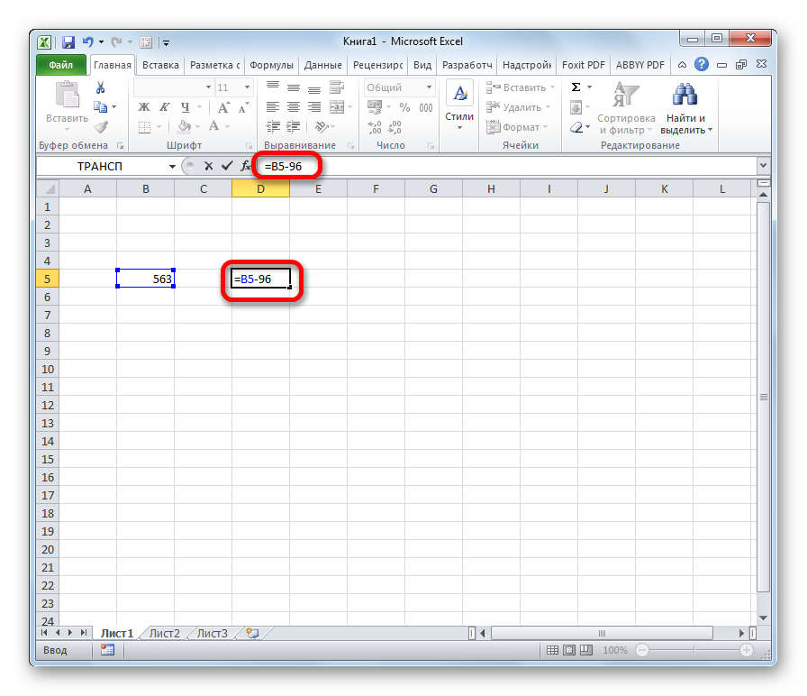
4. To start the calculation, you need to press the “Enter” key. During calculations, the program will subtract the number from the contents of the cell. In the same way, the result will appear in the cell with the formula. Result example:

Example 3: difference between numbers in cells

It is not necessary that the expression even contain one specific number – all actions can be performed only with cells. This is useful when there are many columns in the table and you need to quickly calculate the final result using subtraction.

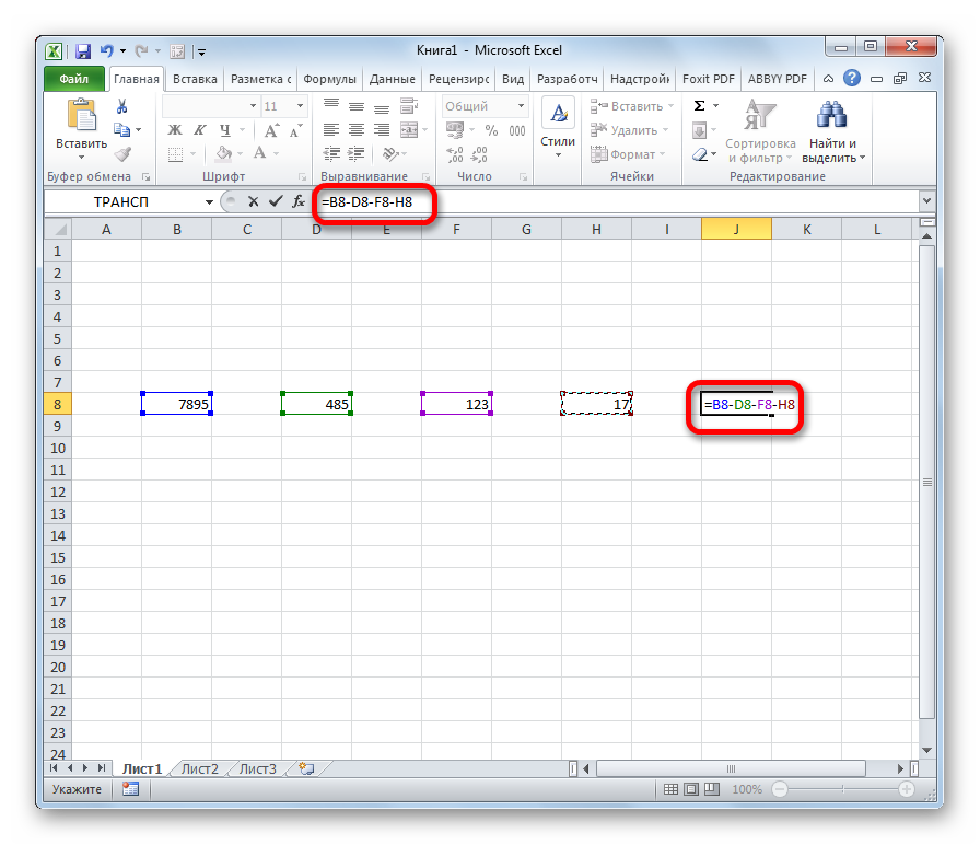
1. The calculation starts with putting an equal sign in the selected cell.
2. After that, you need to find the cell that contains the minuend. It is important not to confuse the parts of the table with each other, because subtraction differs from addition in the strict order in which the expression is written.
3. After clicking on it, the function will have a name in the form of row and column designations, for example, A2, C12, and so on. Put a minus and find in the table a cell with a subtrahend.
4. You also need to click on it, and the expression will become complete – the designation of the subtrahend will automatically fall into it. You can add as many deductibles and actions as you want – the program will automatically calculate everything. Take a look at what the final expression looks like:

5. We press the “Enter” key and we get the difference between the contents of several cells without unnecessary actions in the form of copying or re-entering numbers manually.

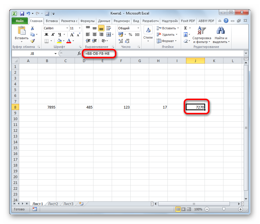
Important! The main rule for using this method is to make sure that the cells in the expression are in the right places.

Example 4: subtracting one column from another

There are cases when you need to subtract the contents of the cells of one column from the cells of another. It’s not uncommon for users to start writing separate formulas for each row, but this is a very time consuming process. To save the time spent writing dozens of expressions, you can subtract one column from another with a single function.

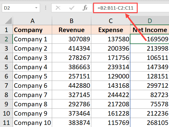
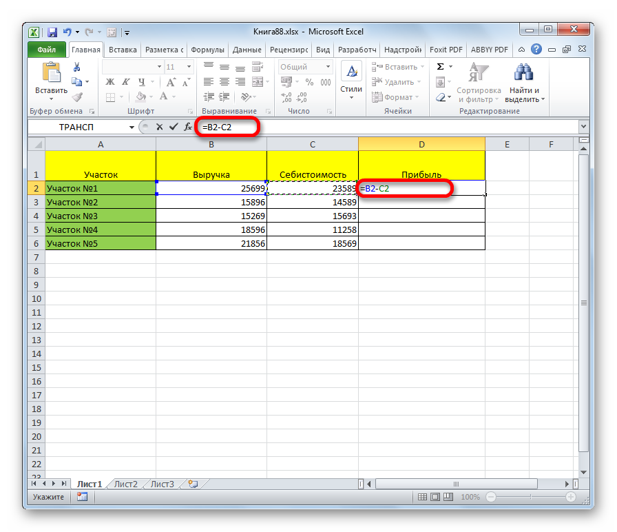
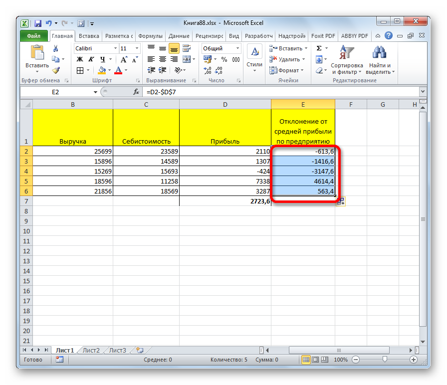
The reasons for using this method may vary, but one of the most common is the need to calculate profit. To do this, you need to subtract the cost of goods sold from the amount of income. Consider the subtraction method using this example:

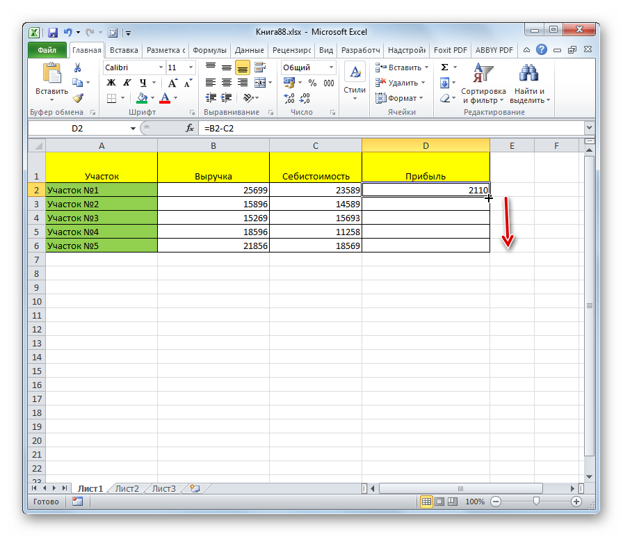
1. It is necessary to double-click on the top cell of an empty column, enter the “=” sign.
2. Next, you need to draw up a formula: select the cell with revenue, put it in the minus function after its designation, and click on the cell with the cost.

Attention! If the cells are selected correctly, you should not click on other elements of the sheet. It is easy not to notice that the minuend or subtrahend has accidentally changed due to such an error.

3. The difference will appear in the cell after pressing the “Enter” key. Before performing the rest of the steps, you need to run the calculation.

4. Take a look at the lower right corner of the selected cell – there is a small square. When you hover over it, the arrow turns into a black cross – this is a fill marker. Now you need to hold down the lower right corner of the cell with the cursor and drag down to the last cell included in the table.

Important! Selecting the lower cells after clamping the outline of the upper cell in other places will not lead to the transfer of the formula to the lines below.

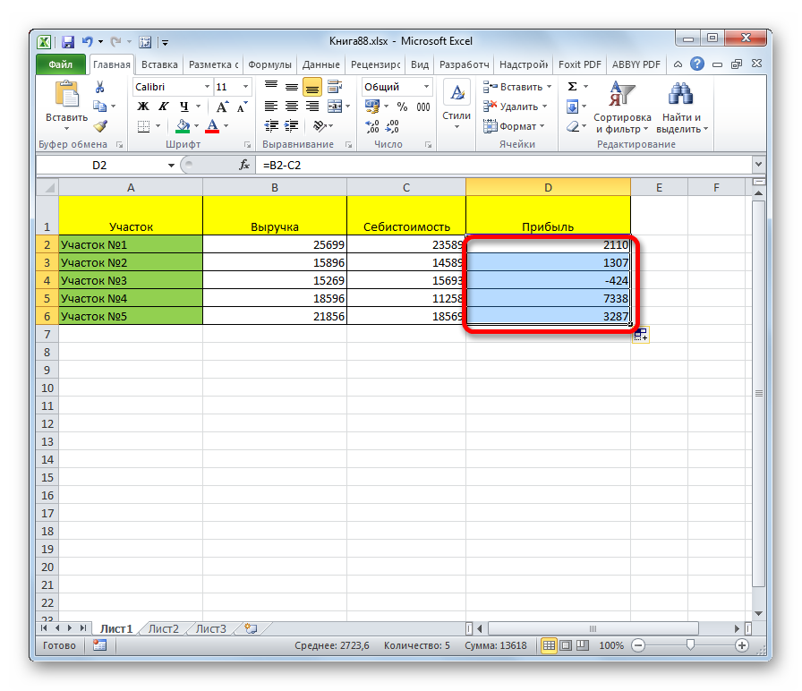
5. The subtraction formula will move to each cell of the column, replacing the minuend and subtrahend with the corresponding designation line. Here’s what it looks like:

Example 5: subtracting a specific number from a column

Sometimes users want only a partial shift to occur when copying, that is, that one cell in the function remains unchanged. This is also possible thanks to the spreadsheet Microsoft Excel.

1. You should start again by choosing a free cell and elements of the expression, putting the signs “=” and “-“. Imagine that in a particular case, the subtrahend must remain unchanged. The formula takes the standard form:

2. Before the notation of the subtrahend cell, letter and number, you need to put dollar signs. This will fix the subtrahend in the formula, will not allow the cell to change.

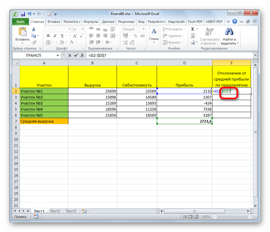
3. Let’s start the calculation by clicking on the “Enter” key, a new value will appear in the first line of the column.
4. Now you can fill in the entire column. It is necessary to hold the marker in the lower right corner of the first cell and select the remaining parts of the column.

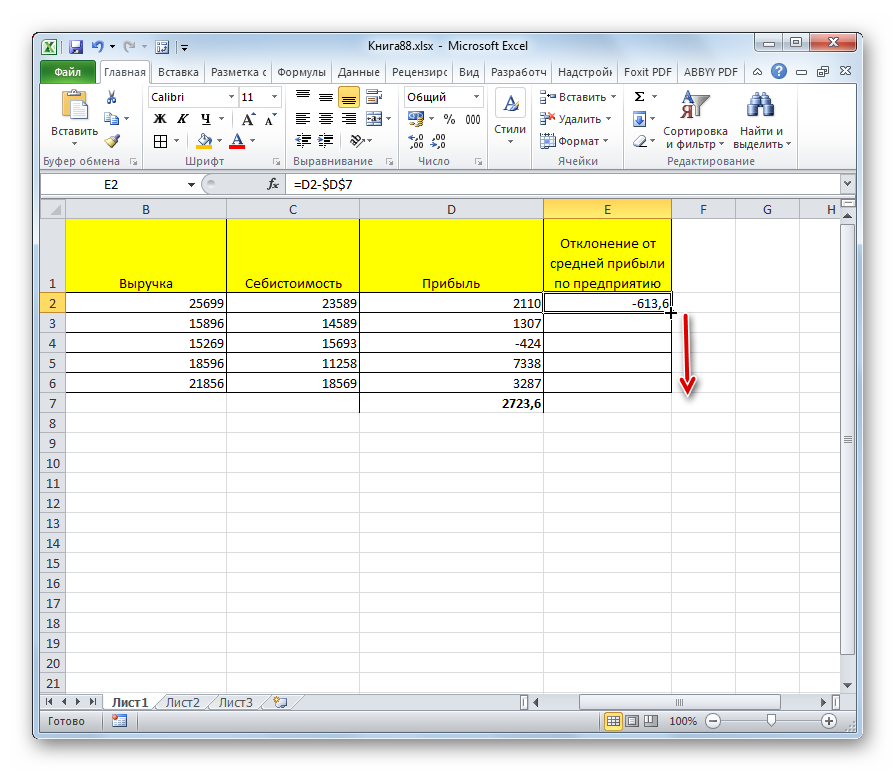
5. The calculation will be carried out with all the necessary cells, while the subtrahend will not change. You can check this by clicking on one of the selected cells – the expression with which it is filled will appear in the function line. The final version of the table looks like this:

A reduced cell can also become a permanent cell – it depends on where to put the “$” signs. The example shown is a special case, the formula does not always have to look like this. The number of expression components can be any.

Subtraction of numbers in intervals

You can subtract a single number from the contents of a column using the SUM function.

1. Select a free cell and open the “Function Manager”.
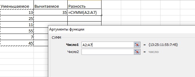
2. You need to find the SUM function and select it. A window will appear for filling the function with values.
3. We select all the cells of the line of the reduced, where there are values, the interval will fall into the line “Number 1”, the next line does not need to be filled.

4. After clicking on the “OK” button, the sum of all the cells of the reduced one will appear in the number selection window in the cell, but this is not the end – you need to subtract.
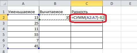
5. Double-click on the cell with the formula and add a minus sign after the closing bracket.
6. Next, you need to select the cell to be subtracted. As a result, the formula should look like this:

7. Now you can press “Enter”, and the desired result will appear in the cell.
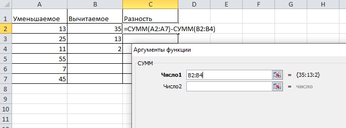
8. Another interval can become subtracted, for this you need to use the SUM function again after the minus. As a result, one interval is subtracted from the other. Let’s slightly supplement the table with the values ​​in the subtrahend column for clarity:

IMSUBTR function

In , this function is called IMNIM.DIFF. This is one of the engineering functions, with its help you can calculate the difference of complex numbers. A complex number consists of real and imaginary units. Despite the fact that there is a plus between the units, this notation is a single number, not an expression. In reality, it is impossible to imagine such a phenomenon, it is purely mathematical. Complex numbers can be represented on the plane as points.

The imaginary difference is the combination of the differences between the real and imaginary parts of a complex number. The result of the subtraction outside the table:

(10+2i)-(7+10i) = 3-8i

10-7 3 =

2i-10i= -8i

1. To carry out calculations, select an empty cell, open the “Function Manager” and find the function IMAGINARY DIFF. It is located in the “Engineering” section.
2. In the number selection window, you need to fill in both lines – each should contain one complex number. To do this, click on the first line, and then – on the first cell with a number, do the same with the second line and cell. The final formula looks like this:

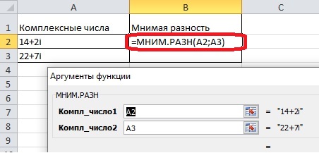
3. Next, press “Enter” and get the result. There is no more than one subtrahend in the formula, you can calculate the imaginary difference of only two cells.

Conclusion

Excel tools make subtraction an easy math operation. The program allows you to perform both the simplest actions with a minus sign, and engage in narrowly focused calculations using complex numbers. Using the methods described above, you can do a lot more while working with tables.