


Contents
When using Microsoft Excel, very often the user does not know in advance how much information will be in the table as a result. Therefore, we do not understand in all situations what range should be covered. After all, a set of cells is a variable concept. To get rid of this problem, it is necessary to make the range generation automatic so that it is based solely on the amount of data that was entered by the user.
Automatically changing cell ranges in Excel
The advantage of automatic ranges in Excel is that they make it much easier to use formulas. In addition, they make it possible to significantly simplify the analysis of complex data that contains a large number of formulas, which include many functions. You can give this range a name, and then it will be updated automatically depending on what data it contains.
How to make automatic range change in Excel
Suppose you are an investor who needs to invest in some object. As a result, we want to get information about how much you can earn in total for the entire time that the money will work for this project. Nevertheless, in order to obtain this information, we need to regularly monitor how much total profit this object brings to us. Make the same report as in this screenshot.
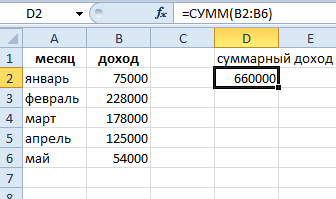
At first glance, the solution is obvious: you just need to sum the whole column. If entries appear in it, the amount will be updated independently. But this method has many disadvantages:
- If the problem is solved in this way, it will not be possible to use the cells included in column B for other purposes.
- Such a table will consume a lot of RAM, which will make it impossible to use the document on weak computers.
Hence, it is necessary to solve this problem through dynamic names. To create them, you must perform the following sequence of actions:
- Go to the “Formulas” tab, which is located in the main menu. There will be a section “Defined names”, where there is a button “Assign a name”, on which we need to click.
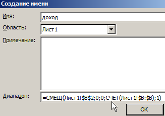
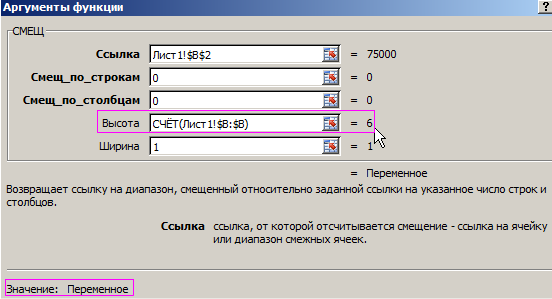
- Next, a dialog box will appear in which you need to fill in the fields as shown in the screenshot. It is important to note that we need to apply the function = DISPLACEMENT together with the function CHECKto create an auto-updating range.

- After that we need to use the function SUM, which uses our dynamic range as an argument.
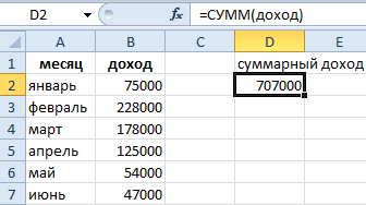
After completing these steps, we can see how the coverage of the cells belonging to the “income” range is updated as we add new elements there.
OFFSET function in Excel
Let’s look at the functions that we recorded in the “range” field earlier. Using the function DISPOSAL we can determine the amount of range given how many cells in column B are filled. The function arguments are as follows:
- Start cell. With this argument, the user can indicate which cell in the range will be considered top left. It will report down and to the right.
- Range offset by rows. Using this range, we set the number of cells by which an offset should occur from the top left cell of the range. You can use not only positive values, but zero and minus. In this case, the displacement may not occur at all, or it will be carried out in the opposite direction.
- Range offset by columns. This parameter is similar to the previous one, only it allows you to set the degree of horizontal shift of the range. Here you can also use both zero and negative values.
- The amount of range in height. In fact, the title of this argument makes it clear to us what it means. This is the number of cells by which the range should increase.
- The value of the range in width. The argument is similar to the previous one, only it concerns the columns.
You don’t need to specify the last two arguments if you don’t need to. In this case, the range value will be only one cell. For example, if you specify the formula =OFFSET(A1;0;0), this formula will refer to the same cell as the one in the first argument. If the vertical offset is set to 2 units, then in this case the cell will refer to cell A3. Now let’s describe in detail what the function means CHECK.
COUNT function in Excel
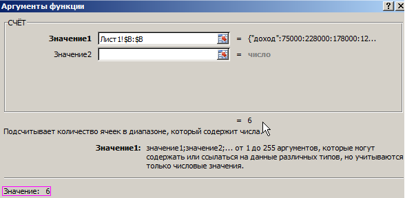
Using the function CHECK we determine how many cells in column B we have filled in total. That is, using two functions, we determine how many cells in the range are filled, and based on the information received, determines the size of the range. Therefore, the final formula will be the following: =СМЕЩ(Лист1!$B$2;0;0;СЧЁТ(Лист1!$B:$B);1)
Let’s take a look at how to correctly understand the principle of this formula. The first argument points to where our dynamic range starts. In our case, this is cell B2. Further parameters have zero coordinates. This suggests that we do not need offsets relative to the top left cell. All we are filling in is the vertical size of the range, which we used the function as CHECK, which determines the number of cells that contain some data. The fourth parameter that we filled in is the unit. Thus we show that the total width of the range should be one column.
Thus, using the function CHECK the user can use the memory as efficiently as possible by loading only those cells that contain some values. Accordingly, there will be no additional errors in the work associated with the poor performance of the computer on which the spreadsheet will work.
Accordingly, in order to determine the size of the range depending on the number of columns, you need to perform a similar sequence of actions, only in this case you need to specify the unit in the third parameter, and the formula in the fourth CHECK.
We see that with the help of Excel formulas, you can not only automate mathematical calculations. This is just a drop in the ocean, but in fact they allow you to automate almost any operation that comes to mind.
Dynamic Charts in Excel
So, in the last step, we were able to create a dynamic range, the size of which completely depends on how many filled cells it contains. Now, based on this data, you can create dynamic charts that will automatically change as soon as the user makes any changes or adds an additional column or row. The sequence of actions in this case is as follows:
- We select our range, after which we insert a chart of the “Histogram with grouping” type. You can find this item in the “Insert” section in the “Charts – Histogram” section.
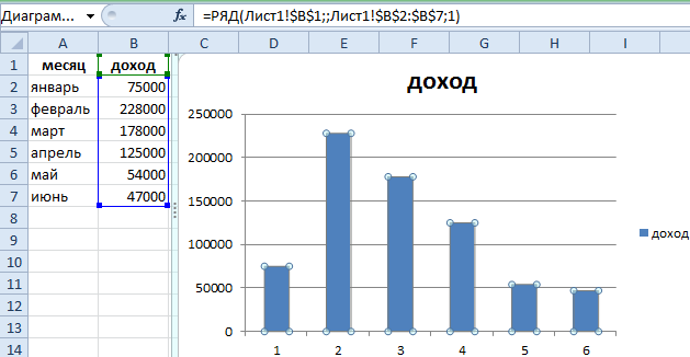
- We make a left mouse click on a random column of the histogram, after which the function =SERIES() will be shown in the function line. In the screenshot you can see the detailed formula.
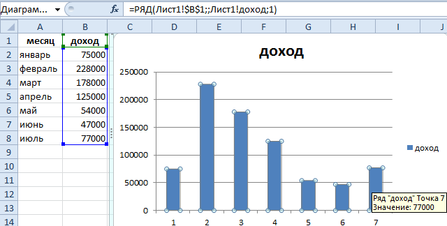
- After that, some changes need to be made to the formula. You need to replace the range after “Sheet1!” to the name of the range. This will result in the following function: =ROW(Sheet1!$B$1;;Sheet1!income;1)
- Now it remains to add a new record to the report to check if the chart is updated automatically or not.
Let’s take a look at our diagram.
Let’s summarize how we did it. In the previous step, we created a dynamic range, the size of which depends on how many elements it contains. To do this, we used a combination of functions CHECK и DISPOSAL. We made this range named, and then we used the reference to this name as the range of our histogram. Which specific range to choose as a data source at the first stage is not so important. The main thing is to replace it with the name of the range later. This way you can save a lot of RAM.
Named ranges and their uses
Let’s now talk in more detail about how to correctly create named ranges and use them to perform the tasks that are set for the Excel user.
By default, we use regular cell addresses in order to save time. This is useful when you need to write a range one or more times. If it needs to be used all the time or it needs to be adaptive, then named ranges should be used. They make creating formulas much easier, and it will not be so difficult for the user to analyze complex formulas that include a large number of functions. Let’s describe some of the steps involved in creating dynamic ranges.
It all starts with naming the cell. To do this, simply select it, and then write the name that we need in the field of its name. It is important that it be easy to remember. There are some restrictions to consider when naming:
- The maximum length is 255 characters. This is quite enough to assign a name that your heart desires.
- The name must not contain spaces. Therefore, if it contains several words, then it is possible to separate them using the underscore character.
If later on other sheets of this file we need to display this value or apply it to perform further calculations, then there is no need to switch to the very first sheet. You can just write down the name of this range cell.
The next step is to create a named range. The procedure is basically the same. First you need to select a range, and then specify its name. After that, this name can be used in all other data operations in Excel. For example, named ranges are often used to define the sum of values.
In addition, it is possible to create a named range using the Formulas tab using the Set Name tool. After we select it, a window will appear where we need to choose a name for our range, as well as specify the area to which it will extend manually. You can also specify where this range will operate: within a single sheet or throughout the book.
If a name range has already been created, then in order to use it, there is a special service called a name manager. It allows not only editing or adding new names, but also deleting them if they are no longer needed.
It should be borne in mind that when using named ranges in formulas, then after deleting it, the formulas will not automatically be overwritten with the correct values. Therefore, errors may occur. Therefore, before deleting a named range, you need to make sure that it is not used in any of the formulas.
Another way to create a named range is to get it from a table. To do this, there is a special tool called “Create from Selection”. As we understand, in order to use it, you must first select the range that we will edit, and then set the place in which we have the headings. As a result, based on this data, Excel will automatically process all the data, and titles will be automatically assigned.
If the title contains several words, Excel will automatically separate them with an underscore.
Thus, we figured out how to create dynamic named ranges and how they allow you to automate work with large amounts of data. As you can see, it is enough to use several functions and the program tools built into the functionality. There is nothing complicated at all, although it may seem so to a beginner at first glance.