How to calculate the percentage of the sum of numbers in Excel

Excel allows you to perform a variety of operations with percentages: determine the percentage of a number, add them together, add a percentage to a number, determine by what percentage the number has increased or decreased, and also perform a huge number of other operations. These skills are very much in demand in life. You constantly have to deal with them, because all discounts, loans, deposits are calculated on their basis. Let’s take a closer look at how to carry out a variety of operations with interest, from the simplest to the most complex.

What is a percentage

Almost all of us understand what interest is and how to calculate it. Let’s repeat this stuff. Let’s imagine that 100 units of a certain product were delivered to the warehouse. Here one unit in this case is equal to one percent. If 200 units of goods were imported, then one percent would be two units, and so on. To get one percent, you need to divide the original figure by one hundred. This is where you can get away with it now.

Calculation of percentage of the amount in Excel

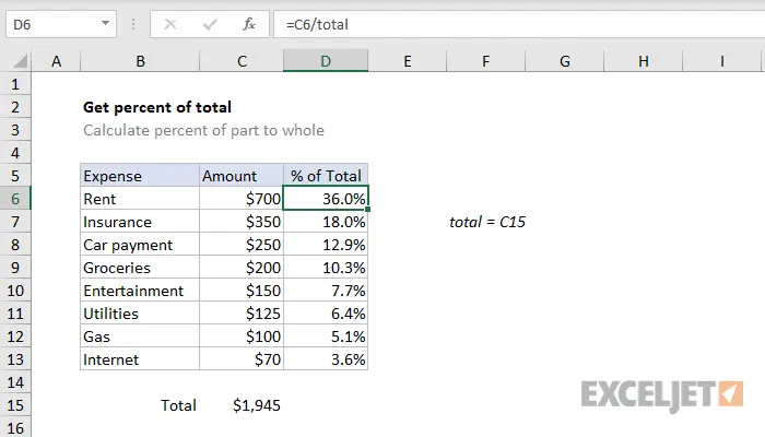
In general, the example described above is already a vivid demonstration of obtaining a percentage value from a larger value (that is, the sum of smaller ones). To better understand this topic, let’s take another example.

You will find out how to quickly determine the percentage of the sum of values ​​using Excel.

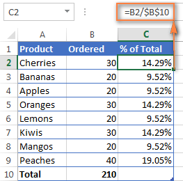
Suppose a table is open on our computer that contains a large range of data and the final information is recorded in one cell. Accordingly, we need to determine what proportion of one position against the background of the total value. In fact, everything must be done in the same way as the previous paragraph, only the link in this case must be turned into an absolute, not a relative one.

For example, if the values ​​are displayed in column B, and the resulting figure is in cell B10, then our formula will look like this.

=B2/$B$10

Let’s analyze this formula in more detail. Cell B2 in this example will change when autofilled. Therefore, its address must be relative. But the address of cell B10 is completely absolute. This means that both the row address and the column address do not change when you drag the formula to other cells.

To turn the link into an absolute one, you must press F4 the required number of times or put a dollar sign to the left of the row and/or column address. 

In our case, we need to put two dollar signs, as shown in the example above.

Here is a picture of the result.

Let’s take a second example. Let’s imagine we have a similar table as in the previous example, only the information is spread over several rows. We need to determine what proportion of the total amount accounts for orders of one product.

The best way to do this is to use the function SUMMESLI. With its help, it becomes possible to sum only those cells that fall under a specific condition. In our example, this is the given product. The results obtained are used to determine the share of the total. 

=SUMIF(range, criteria, sum_range)/total sum

Here, column A contains the names of goods that together form a range. Column B describes information about the summation range, which is the total number of delivered goods. The condition is written in E1, it is the name of the product, which the program focuses on when determining the percentage.

In general, the formula will look like this (given that the grand total will be defined in cell B10).

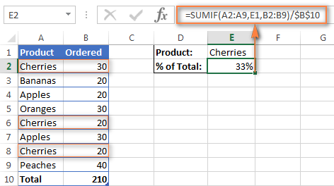
It is also possible to write the name directly into the formula.

=СУММЕСЛИ(A2:A9;»cherries»;B2:B9)/$B$10

If you want to calculate the percentage of several different products from the total, then this is done in two stages:

1. Each item is combined with each other.
2. Then the resulting result is divided by the total value.

So, the formula that determines the result for cherries and apples will be as follows:

=(СУММЕСЛИ(A2:A9;»cherries»;B2:B9)+СУММЕСЛИ(A2:A9;»apples»;B2:B9))/$B$10

How to calculate the percentage of the sum of the values ​​​​of an Excel table

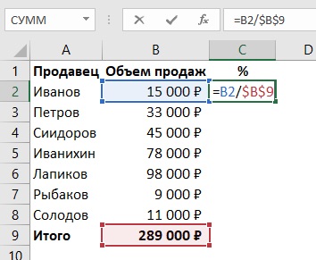
Let’s make such a table with a list of sellers and the volume that he managed to negotiate. At the bottom of the table is the final cell, which records how much they all together were able to sell products. Let’s say we promised three topics, whose percentage of the total turnover is the highest, a bonus. But first you need to understand how many percent of the revenue as a whole falls on each seller.

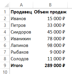
Add an extra column to an existing table.

In cell C2, write the following formula.

=B2/$B$9

As we already know, the dollar sign makes the link absolute. That is, it does not change depending on where the formula is copied or dragged using the autocomplete handle. Without using an absolute reference, it is impossible to make a formula that will compare one value with another specific value, because when shifted down, the formula will automatically become this:

=B3/$B$10

We need to make sure that the first address moves, and the second does not.

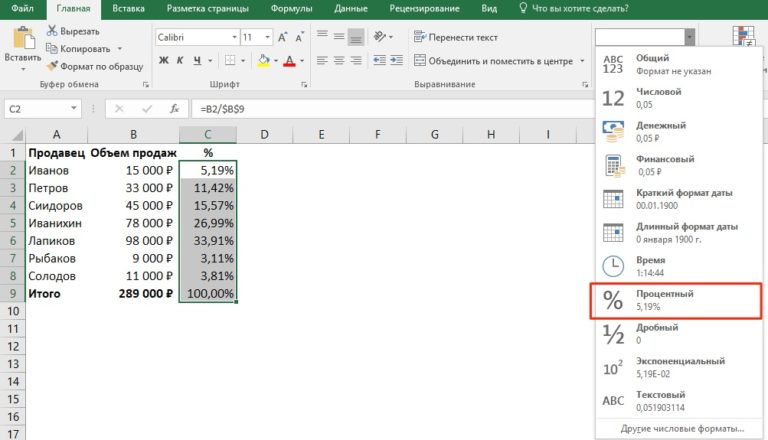
After that, we directly drag the values ​​to the remaining cells of the column using the autocomplete handle.

After applying the percentage format, we get this result.

How to calculate percentage of a number in Excel

To determine what part of a particular number in Excel, you should divide the smaller number by the larger one and multiply everything by 100.

Interest in Excel has its own format. Its main difference is that such a cell automatically multiplies the resulting value by 100 and adds a percent sign. Accordingly, the formula for obtaining a percentage in Excel is even simpler: you just need to divide a smaller number by a larger one. Everything else the program will calculate itself.

Now let’s describe how it works on a real example.

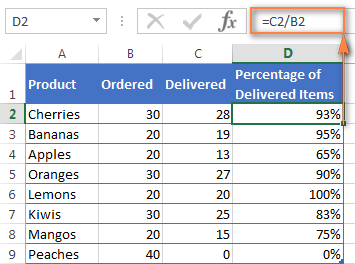
Let’s say you have created a table that shows a specific number of ordered items and a certain number of delivered products. To understand what percentage was ordered, it is necessary (the formula is written based on the fact that the total number is written in cell B, and the delivered goods are in cell C):

1. Divide the number of goods delivered by the total number. To do this, just enter =C2/B2 to the formula bar.
2. Next, this function is copied to the required number of rows using the autocomplete marker. Cells are assigned the format “Percentage”. To do this, click the corresponding button in the “Home” group.
3. If there are too many or too few numbers after the decimal point, you can adjust this setting.

After these simple manipulations, we get a percentage in the cell. In our case, it is listed in column D.

Even if a different formula is used, nothing fundamentally changes in the actions.

The desired number may not be in any of the cells. Then it will have to be entered in the formula manually. It is enough just to write the corresponding number in place of the required argument.

= 20 / 150

How to calculate the percentage of multiple values ​​from the sum of a table

In the previous example, there was a list of the names of the sellers, as well as the number of products sold, which they managed to reach. We needed to determine how significant each individual’s contribution was to the overall earnings of the company.

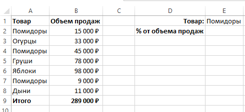
But let’s imagine a different situation. We have a list where the same values ​​are described in different cells. The second column is information on sales volumes. We need to calculate the share of each product in the total revenue, expressed as a percentage.

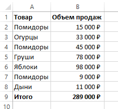
Let’s say we need to figure out what percentage of our total revenue comes from tomatoes, which are distributed across multiple rows in a range. The sequence of actions is as follows:

1. Specify the product on the right.
   

   

2. We make it so that the information in cell E2 is displayed as a percentage. 
3. Apply SUMMESLI to sum the tomatoes and determine the percentage. 

The final formula will be the following.

=СУММЕСЛИ($A$2:$A$8;$E$1;$B$2:$B$8)/B9

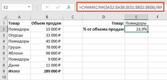
How this formula works

We have applied the function SUMMESLEY, adding the values ​​of two cells, if, as a result of checking for their compliance with a certain condition, Excel returns a value TRUE.

The syntax for this function is very simple. The range of criteria evaluation is written as the first argument. The condition is written in the second place, and the range to be summed is in the third place. 

Optional argument. If you don’t specify it, Excel will use the first one as the third one.

How to add percentages to a number in Excel

In some life situations, the usual structure of expenses may change. It is possible that some changes will have to be made. 

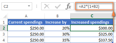
The formula for adding a certain percentage to a number is very simple.

=Value*(1+%)

For example, while on vacation, you might want to increase your entertainment budget by 20%. In this case, this formula will take the following form.

=A1*(1-20%)

Difference between numbers as a percentage in Excel

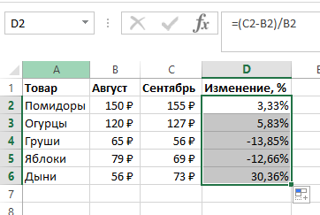
The formula for determining the difference between cells or individual numbers as a percentage has the following syntax.

(B-A)/A

Applying this formula in real practice, you need to clearly understand where to insert which number.

A small example: let’s say you had 80 apples delivered to the warehouse yesterday, while today they brought as many as 100.

Question: how many more were brought today? If you calculate according to this formula, the increase will be 25 percent.

How to find percentage between two numbers from two columns in Excel

To determine the percentage between two numbers from two columns, you must use the formula above. But set others as cell addresses.

Suppose we have prices for the same product. One column contains the larger one, and the second column contains the smaller one. We need to understand the extent to which the value has changed compared to the previous period.

The formula is similar to the one given in the previous example, just in the necessary places you need to insert not cells that are in different rows, but in different columns.

How the formula will look in our case is clearly visible in the screenshot.

It remains to take two simple steps:

1. Set percentage format.
2. Drag the formula to all other cells.

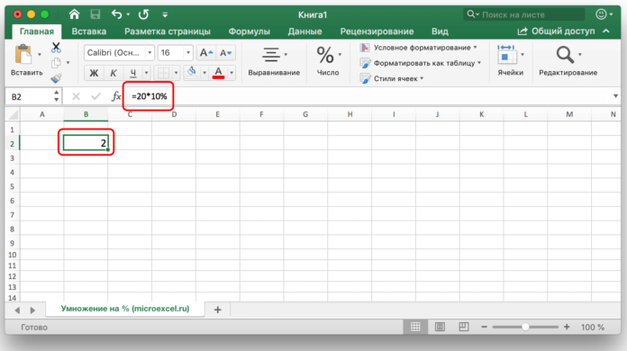
How to multiply by percentage in excel

Sometimes you may need to multiply the contents of cells by a certain percentage in Excel. To do this, you just need to enter a standard arithmetic operation in the form of a cell number or a number, then write an asterisk (*), then write the percentage and put the % sign.

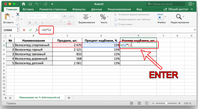
The percentage can also be contained in another cell. In this case, you need to specify the address of the cell containing the percentage as the second multiplier.

How to find the percentage between two numbers from 2 rows in excel

The formula is similar, but instead of a smaller number, you need to give a link to a cell containing a smaller number, and instead of a larger number, respectively.

How to calculate loan interest using Excel

Before compiling a loan calculator, you need to consider that there are two forms of their accrual. The first is called annuity. It implies that every month the amount remains the same.

The second is differentiated, where monthly payments are reduced.

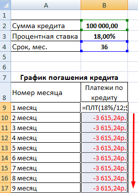
Here is a simple technique on how to calculate annuity payments in Excel.

1. Create a table with initial data.
2. Create a payment table. So far, there will be no exact information in it.
3. Enter formula =ПЛТ($B$3/12; $B$4; $B$2) to the first cell. Here we use absolute references.
   

   

With a differentiated form of payments, the initial information remains the same. Then you need to create a label of the second type.

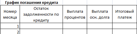
In the first month, the balance of the debt will be the same as the amount of the loan. Next, to calculate it, you need to use the formula =ЕСЛИ(D10>$B$4;0;E9-G9), according to our plate. 

To calculate the interest payment, you need to use this formula: =E9*($B$3/12).

Next, these formulas are entered in the appropriate columns, and then they are transferred to the entire table using the autocomplete marker.