


Contents
Making final totals within an Excel spreadsheet is easy. Therefore, many users are interested in what ways it is possible to sum up intermediate ones within the same table. Of course, you can do everything manually, but since Excel is a program for automating data processing, let’s take a closer look at the methods by which you can entrust this task to a computer.
Requirements for tables for summing up subtotals
Like any automation, subtotaling has its limitations. Therefore, you need to make sure that the table meets certain requirements before you try to add subtotals to it. Here is a short but exhaustive list:
- Each cell must contain information. None should be empty.
- It is forbidden to create a header consisting of several lines. Only one is allowed. It is also important to make sure that the header is on the first row of the spreadsheet sheet.
- The table does not need to be formatted as such. In simple words, there should be a normal range.
The preparatory stage is very important before doing any work. Therefore, you must first make sure that the range meets all these conditions.
The process of calculating subtotals in Excel
Let’s take a quick example to understand how subtotals work. Let’s say you’re a salesperson and you’re writing a report that describes the number of sales of a certain type of product.
Now our task is to determine the revenue for specific categories of furniture sold. Of course, you can do it with a filter. Then it is enough for us to set the criterion by which the information will be selected, but the final values will still have to be determined manually. This causes a lot of inconvenience if there is a lot of data in the cells.
There is another way to accomplish this task – a special command, which is called “Intermediate totals”.
So, we perform a range check to see if they meet the criteria described above. We made sure that the table is a simple range and not a smart table, the column names are described in the first column, the cells contain values of the same format, and that there are no empty cells.
After that, we immediately begin work:
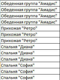
- Focusing on the contents of the cells belonging to the first column, you need to make sure that data of the same type is together.

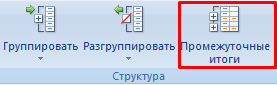
2 - After that, we carry out a random selection of any cell. Next, look at the tape. The tab we are interested in is called “Data”. There is also the button we need, which can be found in the “Structure” group.
3 - After performing these simple actions, a window will pop up in front of us, in which the parameters of the results are set. It has the following fields:
- With every change in In the screenshot, this item is “Name”.
- Operation. Here you need to choose directly the function that is most suitable for the current task. In the situation with us, this is – “Sum”.
- Add totals by. Here you need to specify the columns for which you want to create subtotals.
- Click the OK button to confirm the changes and close the dialog box.
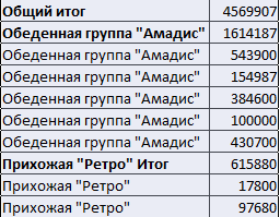
After completing all the operations, the table will look like this.
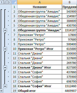
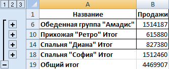
It is possible to collapse rows in subgroups. To do this, you need to click on the minuses, which, as we see in the screenshot, are located on the left side of the screen. Further in our table there will be only intermediate totals.
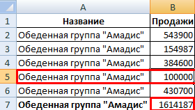
Each time the name changes in the column, it will leave a certain group, and the value of the intermediate will be recalculated.
There are many additional settings for the totals. So that they are separated from the main table by a page break, you must click on the checkbox “End of page between groups”.
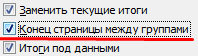
It is also possible to change the location of subtotals. It is possible to place them above the group, and not below it. To do this, uncheck the box next to “Totals under data”.
You can apply more than one aggregate function in subtotals. We have already assigned the “Amount”, but you can add the average sales of specific products.
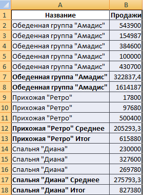
To do this, you need to go back to the “Subtotals” menu. Next, you need to find the item “Replace current”, and then in the “Operation” field, click on the “Average” function.
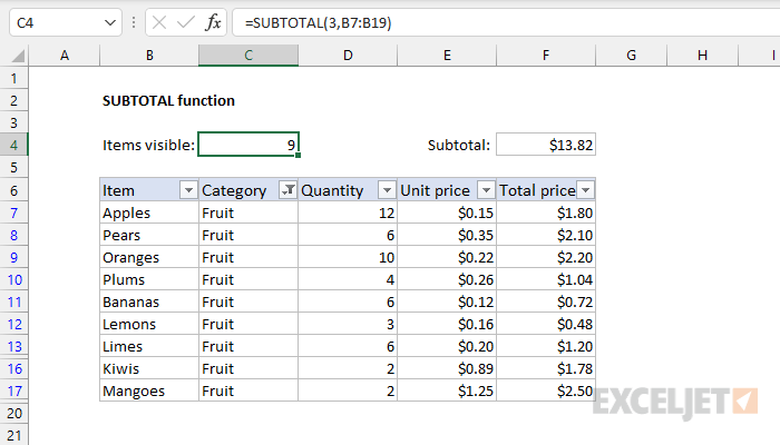
SUBTOTAL function
As the result returned by the function SUBTOTALS serves, as the name implies, an intermediate result. With its help, more flexible creation of subtotals is possible.
Function syntax
The syntax is very simple. First you need to write the number of the function used to summarize. They are numbers ranging from one to eleven. Here is a small list of numbers corresponding to a particular function.

Next come the reference numbers: 1, 2, and so on. Recording the first link is mandatory because it points to the first range of totals. When using this function, you need to take into account the following points:
- It also creates a result for hidden rows. Therefore, if there are any, this factor must be taken into account.
- If certain rows were not added to the filter, the program skips them.
- Counting is carried out exclusively in columns. Therefore, if there is a desire to sum up for a horizontal table, this will not work.
Let’s take a real example of how to use this function correctly.
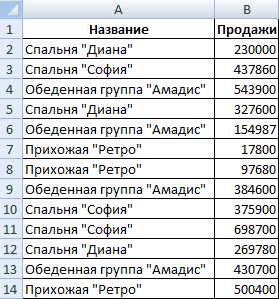
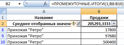
- Add a separate line. We give him a name. Let it be, as an option, “the sum of the selected values”.
- We activate the information filtering so that only those numbers that are located on the same row with the text “Amadis Dining Group” remain in the range.
- Next, enter the formula in cell B2 (or any cell where you can display the intermediate result) = SUBTOTALS (9; B3: B15).
As you can see, a significant advantage of this formula is that it can be used almost anywhere. That is, the table may not be as rigidly standardized as in the previous method.
If it was necessary to calculate the average value, then the formula would look like this.
=SUBTOTAL(1,B3:B15)
In the case of finding the maximum value, the function would be like this.
=SUBTOTAL(4,B3:B15)
In simple words, the user can use this function very flexibly.
SUBTOTAL() function and AutoFilter
Let’s imagine that we have a table with item numbers and their prices.
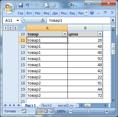
Let’s use the AutoFilter function to display only the rows that describe product number 1. And then let’s use this function to find out the sum of products marked with number 1. Accordingly, we need function 9 or 109.
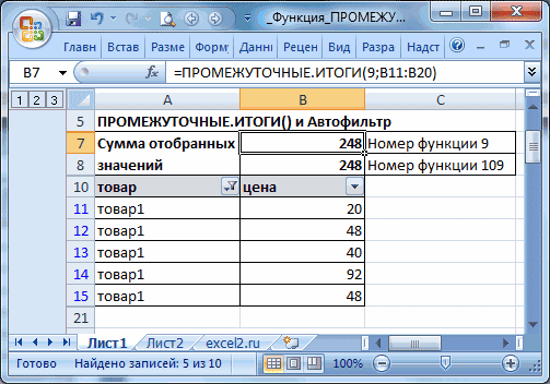
This is another characteristic advantage of this feature. She immediately understands whether the row is hidden by the autofilter or not. If yes, then only the values shown in the table are taken into account. Convenient, isn’t it?
SUBTOTAL() function and Hidden Rows
Let’s say we have the same table that hasn’t had an autofilter applied to it. We will try to simply hide the rows entitled “Product 2” in the standard way. That is, use either the context menu, or go along the path Home – Cells – Format – Hide.
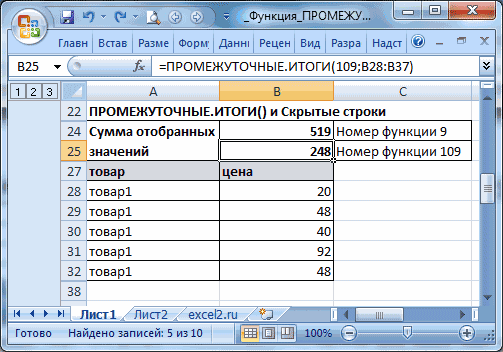
Here the user needs to make sure that the code that matches the hidden lines is used. To put it simply, to search for a subtotal, you must enter the code 109, not 9. The latter option is not sensitive to hidden lines. Therefore, when manually filtering data, you need to use codes starting from 101 and ending with 111. The designations correspond to those described above, you just need to add 100 to them.
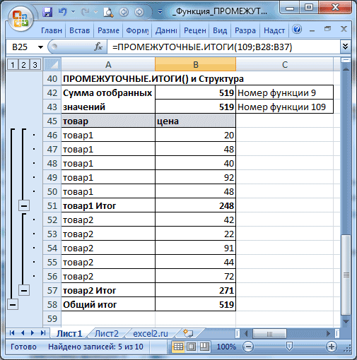
SUBTOTAL() function and Excel Subtotal tool
Let’s now create another table and do subtotals using a special Excel option (not a statistical function, but a special tool described at the beginning of this article).
Now let’s filter the table, leaving only Product1 in it.
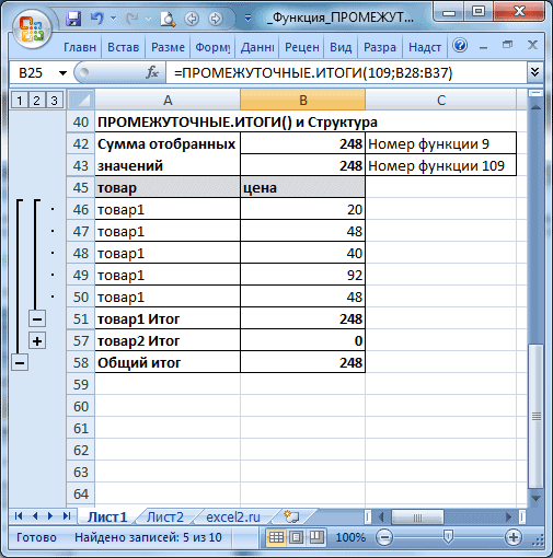
If you use a function that is used in formulas, then it removes all lines that have been removed, no matter what function code is used. In simple words, the result will be the same as if we used an autofilter.
Other Functions
In general, the number of functions that can be used to calculate an intermediate value is sufficient. But it may turn out that you need to include others. Suppose we are faced with the task of calculating not the arithmetic mean, but the geometric mean. This function looks like SRGEOM(), and it is not in the list described above, but it will work out of this situation. To do this, let’s open the same table.
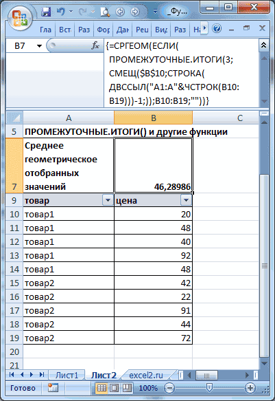
Now, using the autofilter, we leave only one category of rows. So, our task is to force the function SUBTOTALS() determine the geometric mean of the prices of goods with function code 3. The formula itself must be an array formula (that is, taken in curly brackets).
The formula itself will be:
=СРГЕОМ(ЕСЛИ(ПРОМЕЖУТОЧНЫЕ.ИТОГИ(3;СМЕЩ($B$10;СТРОКА(ДВССЫЛ(«A1:A»&ЧСТРОК(B10:B19)))-1;));B10:B19;»»))
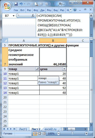
As you can see, we use a combination of functions LINE и INDIRECT in the place where the second argument of the function is located. This way you can ensure that multiple ranges are passed to the second argument. The main thing is to make sure that there is no hidden line, because then, in addition to the cost, the value “Empty text” will be displayed, and it is a function SRGEOM() not taken into account.
Subtotal formula in Excel (examples)
Function SUBTOTALS can be used in a situation where there is a huge amount of data in the table. In this case, after manual configuration through the functionality described at the beginning of the article, it will be possible to display only one part of the table. In this case, all functions will work as if the table was not filtered at all.
The first example is this. Suppose we need to understand what are the interim sales results of the lbanez brand guitar.
Our range looks like this.
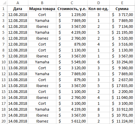
After that, we select the data. After the user uses the filter, some rows will not be displayed. If you use the normal function SUM, then the calculation will be carried out for the entire table.
If we use the function SUBTOTALS, then the result will be shown only for the values remaining after filtering. This difference is visible in this screenshot.
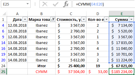
Now we will give an example of selective summation of cells. To do this, in the formula settings window SUBTOTALS (it can be found in the formula input window, which is called by pressing the fx button) you need to check the appropriate checkboxes in the “Add totals by” menu to select the columns for which the summation will be performed. And in order for the formula to be recalculated every time it changes, there is a setting “Whenever you change in”.
Manually writing a subtotal formula
Writing a subtotal formula by hand is no more difficult than writing any other formula. The only thing you need to know is the syntax.
Any formula begins with the = sign, then the name of the function is written directly, the bracket is opened, all arguments are listed separated by a semicolon), and then the bracket is closed.
Subtotals in an Excel PivotTable
Adding subtotals is also possible in a pivot table. To do this, use the “Totals and filters” tab in its parameters. To display totals on the screen for individual values, you must use the filter button (on the right side of the column name).
Thus, there are three methods on how you can add subtotals in Excel, a pivot table, a formula, and the “Structure” group command. Each of them has its own advantages and disadvantages and can be used if it is necessary to automate the process.