


Contents
Communication is a very useful feature in Excel. After all, very often users have to use information from other files. But in some situations, they can do more harm than good. After all, for example, if you send these files by mail, the links are not working. Today we will talk in more detail about what to do to avoid such a problem.
What are relationships in Excel
Relationships in Excel are very often used in conjunction with functions such as VPRto get information from another workbook. It can take the form of a special link that contains the address of not only the cell, but also the book in which the data is located. As a result, such a link looks something like this: =VLOOKUP(A2;'[Sales 2018.xlsx]Report’!$A:$F;4;0). Or, for a simpler representation, represent the address in the following form: ='[Sales 2018.xlsx]Report’!$A1. Let’s analyze each of the link elements of this type:
- [Sales 2018.xlsx]. This fragment contains a link to the file from which you want to get information. It is also called the source.
- Photos. We used the following name, but this is not the name that should be. This block contains the name of the sheet in which you need to find information.
- $A:$F и $A1 – the address of a cell or range containing data that is contained in this document.
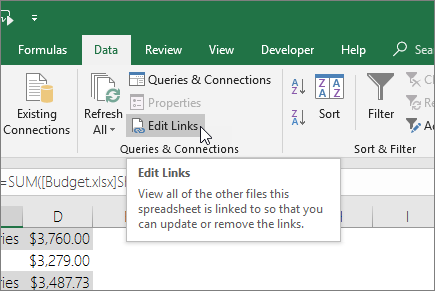
Actually, the process of creating a link to an external document is called linking. After we have registered the address of the cell contained in another file, the contents of the “Data” tab change. Namely, the “Change connections” button becomes active, with the help of which the user can edit the existing connections.
The essence of the problem
As a rule, no additional difficulties arise in order to use links. Even if a situation arises in which the cells change, then all links are automatically updated. But if you already rename the workbook itself or move it to a different address, Excel becomes powerless. Therefore, it produces the following message.
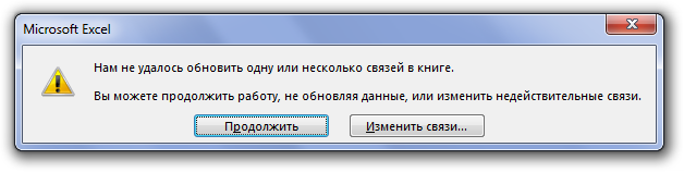
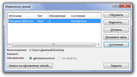
Here, the user has two possible options for how to act in this situation. He can click “Continue” and then the changes will not be updated, or he can click the “Change Associations” button, with which he can update them manually. After we click this button, an additional window will appear in which it will be possible to change the links, indicating where the correct file is located at the moment and what it is called.
In addition, you can edit links through the corresponding button located on the “Data” tab. The user can also find out that the connection is broken by the #LINK error, which appears when Excel cannot access information located at a specific address due to the fact that the address itself is invalid.
How to unlink in excel
One of the simplest methods to solve the situation described above in case you cannot update the location of the linked file yourself is to delete the link itself. This is especially easy to do if the document contains only one link. To do this, you must perform the following sequence of steps:
- Open the “Data” menu.
- We find the section “Connections”, and there – the option “Change connections”.
- After that, click on “Unlink”.
If you intend to mail this book to another person, it is highly recommended that you do so in advance. After all, after deleting the links, all the values that are contained in another document will be automatically loaded into the file, used in formulas, and instead of the cell address, the information in the corresponding cells will simply be transformed into values.
How to unlink all books
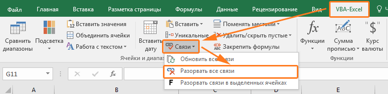
But if the number of links becomes too large, manually deleting them can take a long time. To solve this problem in one go, you can use a special macro. It is in the VBA-Excel addon. You need to activate it and go to the tab of the same name. There will be a “Links” section, in which we need to click on the “Break all links” button.
VBA code
If it is not possible to activate this add-on, you can create a macro yourself. To do this, open the Visual Basic editor by pressing the Alt + F11 keys, and write the following lines in the code entry field.
Sub UnlinkWorkBooks()
Dim WbLinks
Dim and As Long
Select Case MsgBox(“All references to other books will be removed from this file, and formulas referring to other books will be replaced with values.” & vbCrLf & “Are you sure you want to continue?”, 36, “Unlink?”)
Case 7′ No
Exit Sub
End Select
WbLinks = ActiveWorkbook.LinkSources(Type:=xlLinkTypeExcelLinks)
If Not IsEmpty(WbLinks) Then
For i = 1 To UBound(WbLinks)
ActiveWorkbook.BreakLink Name:=WbLinks(i), Type:=xlLinkTypeExcelLinks
Next
else
MsgBox “There are no links to other books in this file.”, 64, “Links to other books”
End If
End Sub
How to break ties only in the selected range
From time to time, the number of links is very large, and the user is afraid that after deleting one of them, it will not be possible to return everything back if some was superfluous. But this is a problem that is easy to avoid. To do this, you need to select the range in which to delete links, and then delete them. To do this, you must perform the following sequence of actions:
- Select the dataset that needs to be modified.
- Install the VBA-Excel add-on, and then go to the appropriate tab.
- Next, we find the “Links” menu and click on the “Break links in the selected ranges” button.
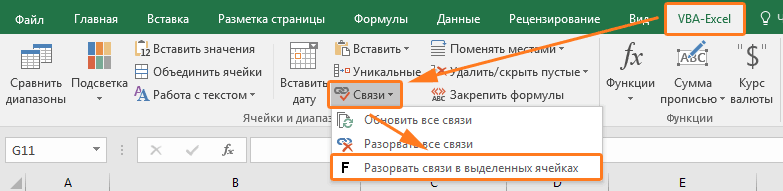
After that, all links in the selected set of cells will be deleted.
What to do if the ties are not broken
All of the above sounds good, but in practice there are always some nuances. For example, there may be a situation where ties are not broken. In this case, a dialog box still appears stating that it is not possible to automatically update the links. What to do in this situation?
- First, you need to check if any information is contained in the named ranges. To do this, press the key combination Ctrl + F3 or open the “Formulas” tab – “Name Manager”. If the file name is full, then you just need to edit it or remove it altogether. Before deleting named ranges, you need to copy the file to some other location so that you can return to the original version if the wrong steps were taken.
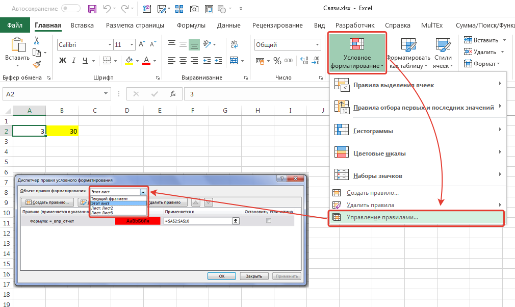
- If you can’t solve the problem by removing names, you can check conditional formatting. Cells in another table can be referenced in conditional formatting rules. To do this, find the corresponding item on the “Home” tab, and then click on the “File Management” button.

Normally, Excel doesn’t give you the ability to give the address of other workbooks in conditional formatting, but you do if you refer to a named range with a reference to another file. Usually, even after the link is removed, the link remains. There is no problem in removing such a link, because the link is in fact not working. Therefore, nothing bad will happen if you remove it.
You can also use the “Data Check” function to find out if there are any unnecessary links. Links usually remain if the “List” type of data validation is used. But what to do if there are a lot of cells? Is it really necessary to check each of them sequentially? Of course not. After all, it will take a very long time. Therefore, you need to use a special code to significantly save it.
Option Explicit
‘—————————————————————————————
‘ Author : The_Prist(Shcherbakov Dmitry)
‘ Professional development of applications for MS Office of any complexity
‘ Conducting trainings on MS Excel
‘ https://www.excel-vba.ru
‘ [email protected]
‘WebMoney—R298726502453; Yandex.Money — 41001332272872
‘ Purpose:
‘—————————————————————————————
Sub FindErrLink()
‘we need to look in the Data -Change links link to the source file
‘and put the keywords here in lowercase (part of the file name)
‘asterisk just replaces any number of characters so you don’t have to worry about the exact name
Const sToFndLink$ = “*sales 2018*”
Dim rr As Range, rc As Range, rres As Range, s$
‘define all cells with data validation
On Error Resume Next
Set rr = ActiveSheet.UsedRange.SpecialCells(xlCellTypeAllValidation)
If rr Is Nothing Then
MsgBox “There are no cells with data validation on the active sheet”, vbInformation, “www.excel-vba.ru”
Exit Sub
End If
On Error GoTo 0
‘check each cell for links
For Each rc In rr
‘just in case, we skip errors – this can also happen
‘but our connections must be without them and they will definitely be found
s = «»
On Error Resume Next
s = rc.Validation.Formula1
On Error GoTo 0
‘found – we collect everything in a separate range
If LCase(s) Like sToFndLink Then
If rres Is Nothing Then
Set rres = rc
else
Set rres = Union(rc, rres)
End If
End If
Next
‘if there is a connection, select all cells with such data checks
If Not rres Is Nothing Then
rres.Select
‘ rres.Interior.Color = vbRed ‘if you want to highlight with color
End If
End Sub
It is necessary to make a standard module in the macro editor, and then insert this text there. After that, call the macro window using the key combination Alt + F8, and then select our macro and click on the “Run” button. There are a few things to keep in mind when using this code:
- Before you search for a link that is no longer relevant, you must first determine what the link through which it is created looks like. To do this, go to the “Data” menu and find the “Change Links” item there. After that, you need to look at the file name, and specify it in quotes. For example, like this: Const sToFndLink$ = “*sales 2018*”
- It is possible to write the name not in full, but simply replace unnecessary characters with an asterisk. And in quotes, write the file name in small letters. In this case, Excel will find all files that contain such a string at the end.
- This code is only able to check for links in the sheet that is currently active.
- With this macro, you can only select the cells that it has found. You have to delete everything manually. This is a plus, because you can double-check everything again.
- You can also make the cells highlighted in a special color. To do this, remove the apostrophe before this line. rres.Interior.Color = vbRed
Usually, after you complete the steps described in the instructions above, there should be no more unnecessary connections. But if there are some of them in the document and you are unable to remove them for one reason or another (a typical example is the security of data in a sheet), then you can use a different sequence of actions. This instruction is valid only for versions 2007 and higher.
- We create a backup copy of the document.
- Open this document using the archiver. You can use any that supports the ZIP format, but WinRar will also work, as well as the one built into Windows.
- In the archive that appears, you need to find the xl folder, and then open externalLinks.
- This folder contains all external links, each of which corresponds to a file of the form externalLink1.xml. All of them are only numbered, and therefore the user does not have the opportunity to understand what kind of connection this is. To understand what kind of connection, you need to open the _rels folder, and look at it there.
- After that, we remove all or specific links, based on what we learn in the externalLinkX.xml.rels file.
- After that, we open our file using Excel. There will be information about an error like “Error in part of the content in the Book.” We give consent. After that, another dialog will appear. We close it.
After that, all links should be removed.