How to compare two lists in Excel

Excel is an efficient data processing program. And one of the methods of information analysis is the comparison of two lists. If you correctly compare two lists in Excel, organizing this process will be very easy. It is enough just to follow some of the points that will be discussed today. The practical implementation of this method depends entirely on the needs of the person or organization at a particular moment. Therefore, several possible cases should be considered.

Comparing two lists in Excel

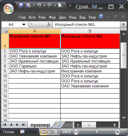
Of course, you can compare two lists manually. But it will take a long time. Excel has its own intelligent toolkit that will allow you to compare data not only quickly, but also to get information that is not so easy to get with your eyes. Suppose we have two columns with coordinates A and B. Some values ​​are repeated in them.

Formulation of the problem

So we need to compare these columns. The procedure for comparing two documents is as follows:

1. If the unique cells of each of these lists are the same, and the total number of unique cells is the same, and the cells are the same, then these lists can be considered the same. The order in which the values ​​in this list are stacked does not matter so much.
2. We can talk about partial coincidence of lists if the unique values ​​themselves are the same, but the number of repetitions is different. Therefore, such lists may contain a different number of elements.
3. The fact that the two lists do not match is indicated by a different set of unique values.

All these three conditions simultaneously are the conditions of our problem.

The solution of the problem

Let’s generate two dynamic ranges to make it easier to compare lists. Each of them will correspond to each of the lists.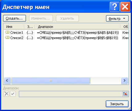

To compare two lists, do the following:

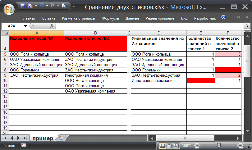
1. In a separate column, we create a list of unique values ​​that are specific to both lists. For this we use the formula: ЕСЛИОШИБКА(ЕСЛИОШИБКА( ИНДЕКС(Список1;ПОИСКПОЗ(0;СЧЁТЕСЛИ($D$4:D4;Список1);0)); ИНДЕКС(Список2;ПОИСКПОЗ(0;СЧЁТЕСЛИ($D$4:D4;Список2);0))); «»). The formula itself must be written as an array formula.
2. Let’s determine how many times each unique value occurs in the data array. Here are the formulas for doing this: =COUNTIF(List1,D5) and =COUNTI(List2,D5).
3. If both the number of repetitions and the number of unique values ​​are the same in all lists that are included in these ranges, then the function returns the value 0. This indicates that the match is XNUMX%. In this case, the headings of these lists will acquire a green background.
4. If all unique content is in both lists, then returned by formulas =СЧЁТЕСЛИМН($D$5:$D$34;»*?»;E5:E34;0) и =СЧЁТЕСЛИМН($D$5:$D$34;»*?»;F5:F34;0) the value will be zero. If E1 does not contain zero, but such a value is contained in cells E2 and F2, then in this case the ranges will be recognized as matching, but only partially. In this case, the headings of the corresponding lists will turn orange.
5. And if one of the formulas described above returns a non-zero value, the lists will be completely non-matching.

This is the answer to the question of how to analyze columns for matches using formulas. As you can see, with the use of functions, you can implement almost any task that, at first glance, is not related to mathematics.

Example Testing

In our version of the table, there are three types of lists of each type described above. It has partially and completely matching, as well as non-matching.

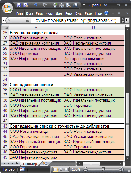
To compare data, we use the range A5:B19, in which we alternately insert these pairs of lists. About what will be the result of the comparison, we will understand by the color of the original lists. If they are completely different, then it will be a red background. If part of the data is the same, then yellow. In the case of complete identity, the corresponding headings will be green. How to make a color depending on what the result is? This requires conditional formatting.

Finding differences in two lists in two ways

Let’s describe two more methods for finding differences, depending on whether the lists are synchronous or not.

Option 1. Synchronous Lists

This is an easy option. Suppose we have such lists.

To determine how many times the values ​​did not converge, you can use the formula: =SUMPRODUCT(—(A2:A20<>B2:B20)). If we got 0 as a result, this means that the two lists are the same.

Option 2: Shuffled Lists

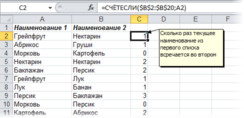
If the lists are not identical in the order of the objects they contain, you need to apply a feature such as conditional formatting and colorize duplicate values. Or use the function COUNTIF, using which we determine how many times an element from one list occurs in the second.

How to compare 2 columns row by row

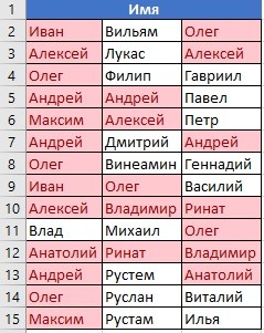
When we compare two columns, we often need to compare information that is in different rows. To do this, the operator will help us IF. Let’s take a look at how it works in practice. To do this, we present several illustrative situations.

Example. How to compare 2 columns for matches and differences in one row

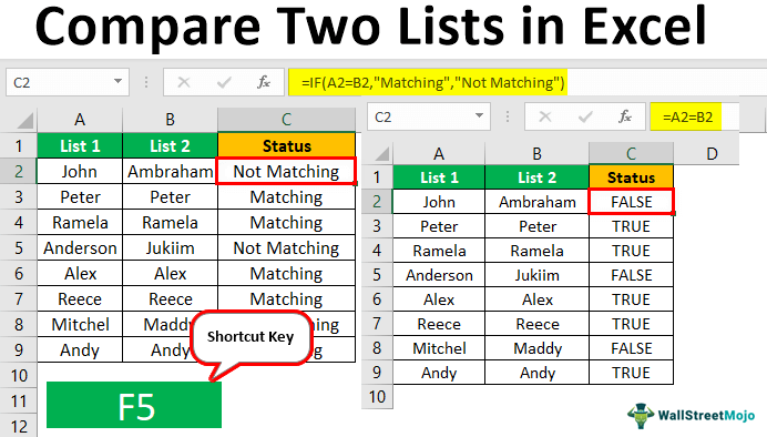
To analyze whether the values ​​that are in the same row but different columns are the same, we write the function IF. The formula is inserted into each row placed in the auxiliary column where the results of data processing will be displayed. But it is not at all necessary to prescribe it in each row, just copy it into the remaining cells of this column or use the autocomplete marker.

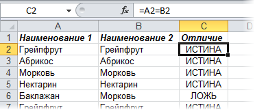
We should write down such a formula to understand whether the values ​​in both columns are the same or not: =IF(A2=B2, “Match”, “”). The logic of this function is very simple: it compares the values ​​in cells A2 and B2, and if they are the same, it displays the value “Coincide”. If the data is different, it does not return any value. You can also check the cells to see if there is a match between them. In this case, the formula used is: =IF(A2<>B2, “Do not match”, “”). The principle is the same, first the check is carried out. If it turns out that the cells meet the criterion, then the value “Does not match” is displayed.

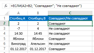
It is also possible to use the following formula in the formula field to display both “Match” if the values ​​are the same, and “Do not match” if they are different: =IF(A2=B2; “Match”, “Do not match”). You can also use the inequality operator instead of the equality operator. Only the order of the values ​​that will be displayed in this case will be slightly different: =IF(A2<>B2, “Do not match”, “Coincide”). After using the first version of the formula, the result will be as follows.

This variation of the formula is case insensitive. Therefore, if the values ​​in one column differ from others only in that they are written in capital letters, then the program will not notice this difference. To make the comparison case-sensitive, you need to use the function in the criteria EXACT. The rest of the arguments are left unchanged: =IF(EXACT(A2,B2), “Match”, “Unique”).

How to compare multiple columns for matches in one row

It is possible to analyze the values ​​in the lists according to a whole set of criteria:

1. Find those rows that have the same values ​​everywhere.
2. Find those rows where there are matches in just two lists.

Let’s look at a few examples of how to proceed in each of these cases.

Example. How to find matches in one row in multiple columns of a table

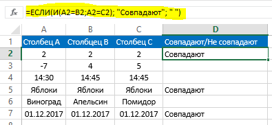
Suppose we have a series of columns that contain the information we need. We are faced with the task of determining those rows in which the values ​​are the same. To do this, you need to use the following formula: =IF(AND(A2=B2,A2=C2), “match”, ” “).

If there are too many columns in the table, then you just need to use it together with the function IF operator COUNTIF: =IF(COUNTIF($A2:$C2,$A2)=3;”match”;” “). The number used in this formula indicates the number of columns to check. If it differs, then you need to write as much as is true for your situation.

Example. How to find matches in one row in any 2 columns of a table

Let’s say we need to check if the values ​​in one row match in two columns from those in the table. To do this, you need to use the function as a condition OR, where alternately write the equality of each of the columns to the other. Here is an example.

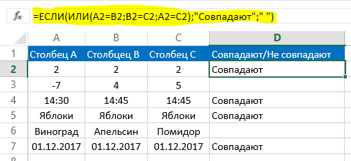
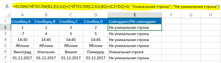
We use this formula: =ЕСЛИ(ИЛИ(A2=B2;B2=C2;A2=C2);”Совпадают”;” “). There may be a situation when there are a lot of columns in the table. In this case, the formula will be huge, and it may take a lot of time to select all the necessary combinations. To solve this problem, you need to use the function COUNTIF: =IF(COUNTIF(B2:D2,A2)+COUNTIF(C2:D2,B2)+(C2=D2)=0; “Unique string”; “Not unique string”)

We see that in total we have two functions COUNTIF. With the first one, we alternately determine how many columns have a similarity to A2, and with the second one, we check the number of similarities with the value of B2. If, as a result of calculating by this formula, we get a zero value, this indicates that all rows in this column are unique, if more, there are similarities. Therefore, if as a result of calculating by two formulas and adding the final results we get a zero value, then the text value “Unique string” is returned, if this number is greater, it is written that this string is not unique.

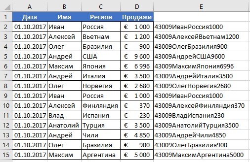
How to compare 2 columns in Excel for matches

Now let’s take an example. Let’s say we have a table with two columns. You need to check if they match. To do this, you need to apply the formula, where the function will also be used IF, and the operator COUNTIF: =IF(COUNTIF($B:$B,$A5)=0, “No matches in column B”, “There are matches in column B”)

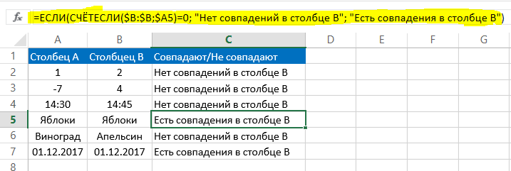
No further action is required. After calculating the result by this formula, we get if the value of the third argument of the function IF matches. If there are none, then the contents of the second argument.

How to compare 2 columns in Excel for matches and highlight with color

To make it easier to visually identify matching columns, you can highlight them with a color. To do this, you need to use the “Conditional Formatting” function. Let’s see in practice.

Finding and highlighting matches by color in multiple columns

To determine the matches and highlight them, you must first select the data range in which the check will be carried out, and then open the “Conditional Formatting” item on the “Home” tab. There, select “Duplicate Values” as the cell selection rule.

After that, a new dialog box will appear, in which in the left pop-up list we find the option “Repeating”, and in the right list we select the color that will be used for the selection. After we click the “OK” button, the background of all cells with similarities will be selected. Then just compare the columns by eye.

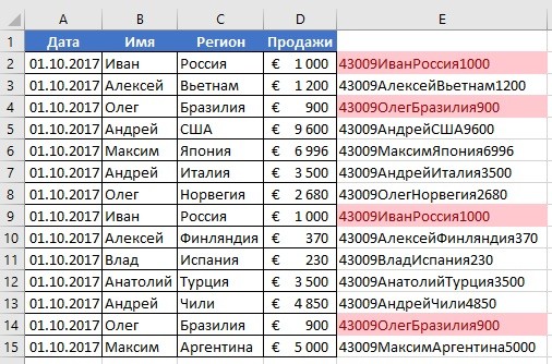
Finding and highlighting matching lines

The technique for checking if strings match is slightly different. First, we need to create an additional column, and there we will use the combined values ​​using the & operator. To do this, you need to write a formula of the form: =A2&B2&C2&D2.

We select the column that was created and contains the combined values. Next, we perform the same sequence of actions that is described above for the columns. Duplicate lines will be highlighted in the color you specify.

We see that there is nothing difficult in looking for repetitions. Excel contains all the necessary tools for this. It is important to just practice before putting all this knowledge into practice.