


Contents
Some Excel users have a problem that the grid on the sheet suddenly disappears. This at least looks ugly, and also adds a lot of inconvenience. After all, these lines help to navigate the contents of the table. Of course, in some situations it makes sense to abandon the grid. But this is only useful when the user himself needs it. Now you do not need to study special e-books on how to solve this problem. Read on and you will see that everything is much easier than it seems.
How to Hide and Restore the Grid on an Entire Excel Sheet
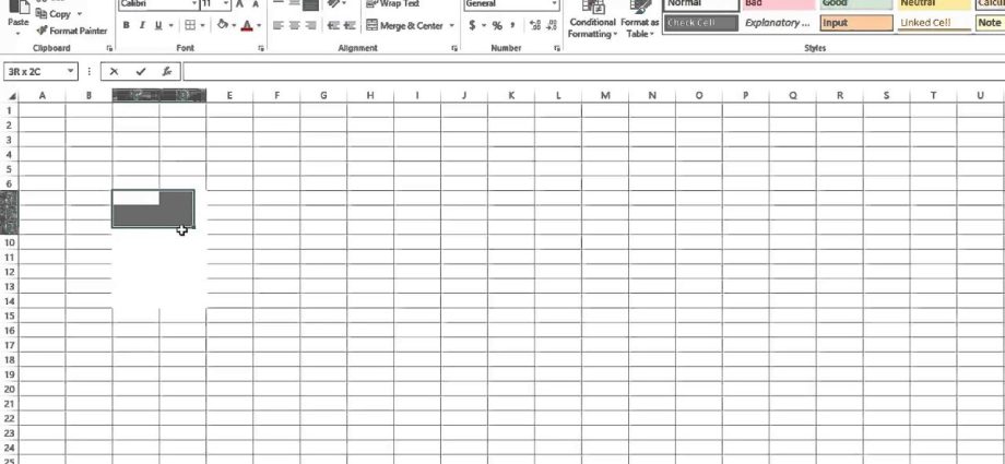
The sequence of actions performed by the user may differ depending on the version of the office suite. An important clarification: this is not about the borders of the cells, but about the reference lines that separate the cells throughout the document.
Excel version 2007-2016
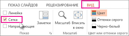
Before we understand how to restore the grid to the entire sheet, we first need to figure out how it happened that it disappeared. A special option on the “View” tab, which is called “Grid”, is responsible for this. If you uncheck this item, the grid will automatically be removed. Accordingly, to restore the document grid, you must check this box.
There is another way. You need to go to the Excel settings. They are located in the “File” menu in the “Options” block. Next, open the “Advanced” menu, and uncheck the “Show grid” checkbox if we want to turn off the display of the grid or check it if we want to return it.
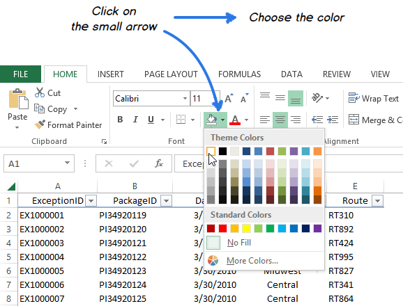
There is another way to hide the grid. To do this, you need to make its color white or the same as the color of the cells. Not the best method to do this, but it might work. In turn, if the color of the lines is already white, then it is necessary to correct it for any other that will be clearly visible.
By the way, take a look. It is possible that there is a different color for the borders of the grid, only it is barely noticeable due to the fact that there are so many shades of white.
Excel version 2000-2003
In older versions of Excel, hiding and showing the grid is more complicated than in newer versions. To do this, follow these steps:
- Open the “Service” menu.
- Go to “Settings”.
- A window will appear in which we need to open the “View” tab.
- Next, we look for a section with window parameters, where we uncheck the box next to the “Grid” item.
Also, as with newer versions of Excel, the user can choose white to hide the grid, or black (or anything that contrasts well with the background) to show it.
Excel provides the ability, among other things, to hide the grid on several sheets or in the entire document. To do this, you must first select the appropriate sheets, and then perform the operations described above. You can also set the line color to “Auto” to display the grid.
How to hide and re-display the cell range grid
Grid lines are used not only to mark the boundaries of cells, but also to align different objects. For example, to make it easier to position the graph relative to the table. So you can achieve a more aesthetic effect. In Excel, unlike other office programs, it is possible to print grid lines. Thus, you can customize their display not only on the screen, but also on print.
As we already know, to display grid lines on the screen, you just need to go to the “View” tab and check the corresponding box.
Accordingly, to hide these lines, simply uncheck the corresponding box.
Grid Display on a Filled Range
You can also show or hide the grid by modifying the Fill Color value. By default, if it is not set, the grid is displayed. But as soon as it is changed to white, the grid borders are automatically hidden. And you can return them by selecting the “No fill” item.
Grid printing
But what do you need to do to print these lines on a sheet of paper? In this case, you need to activate the “Print” option. To do this, you must follow the following instructions:
- First, select the sheets that will be affected by the changes. You can find out that several sheets were selected at once by the [Group] symbol, which will appear on the sheet header. If suddenly the sheets were selected incorrectly, you can cancel the selection by left-clicking on any of the existing sheets.
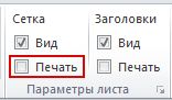
- Open the “Page Layout” tab, on which we are looking for the “Sheet Options” group. There will be a corresponding function. Find the “Grid” group and check the box next to the “Print” item.

Often users encounter this problem: they open the Page Layout menu, but the checkboxes that need to be activated do not work. In simple words, it is not possible to activate or deactivate the corresponding functions.
To solve this, you need to change the focus to another object. The reason for this problem is that the current selection is not a sheet, but a graph or image. Also, the necessary checkboxes appear if you deselect this object. After that, we put the document to print and check. This can be done using the key combination Ctrl + P or using the corresponding menu item “File”.
You can also activate the preview and see how the grid lines will be printed before they appear on paper. To do this, press the combination Ctrl + F2. There you can also change the cells that will be printed. For example, a person might want to print gridlines around cells that don’t have any values. In such a case, the appropriate addresses must be added to the range to be printed.
But for some users, after performing these steps, the grid lines still do not appear. This is because draft mode is enabled. You need to open the “Page Setup” window and uncheck the corresponding box on the “Sheet” tab. If these steps did not help, then the reason may lie in the printer driver. Then a good solution would be to install the factory driver, which can be downloaded from the official website of the manufacturer of this device. The fact is that the drivers that the operating system installs automatically do not always work well.