Creating a Pareto Chart in Excel

The Pareto principle, named after the Italian economist Vilfredo Pareto, states that 80% of problems can be caused by 20% of causes. The principle can be very useful or even life-saving information when you have to choose which of the many problems to solve first, or if the elimination of problems is complicated by external circumstances.

For example, you have just been asked to lead a team that is having difficulty working on a project to point them in the right direction. You ask team members what were their main obstacles in achieving their goals and targets. They make a list that you analyze and find out what were the main causes of each of the problems that the team encountered, trying to see the commonalities.

All detected causes of problems are arranged according to the frequency of their occurrence. Looking at the numbers, you find that the lack of communication between project implementers and project stakeholders is the root cause of the top 23 problems that the team faces, while the second biggest problem is access to the necessary resources (computer systems, equipment, etc.). .) resulted in only 11 associated complications. Other problems are isolated. It is clear that by solving the communication problem, a huge percentage of problems can be eliminated, and by solving the problem of access to resources, almost 90% of the obstacles in the team’s path can be resolved. Not only have you figured out how to help the team, you’ve just done a Pareto analysis.

Doing all this work on paper will probably take a certain amount of time. The process can be greatly accelerated using the Pareto chart in Microsoft Excel.

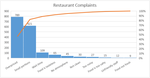
Pareto charts are a combination of a line chart and a histogram. They are unique in that they usually have one horizontal axis (category axis) and two vertical axes. The chart is useful for prioritizing and sorting data.

My task is to help you prepare data for the Pareto chart and then create the chart itself. If your data is already prepared for the Pareto chart, then you can proceed to the second part.

Today we will analyze a problematic situation in a company that regularly reimburses employees for expenses. Our task is to find out what we spend the most on and understand how we can reduce these costs by 80% using a quick Pareto analysis. We can find out what costs account for 80% of refunds and prevent high costs in the future by changing the policy to use wholesale prices and discuss employee costs.

Part One: Prepare Data for the Pareto Chart

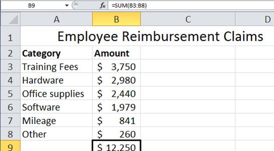
1. Organize your data. In our table, there are 6 categories of cash compensation and amounts claimed by employees.
2. Sort the data in descending order. Check that columns are selected А и Вto sort correctly.
3. Column Sum Amount (number of expenses) is calculated using the function SUM (SUM). In our example, in order to get the total amount, you need to add the cells from V3 to V8.

Hotkeys: To sum a range of values, select a cell B9 and press Alt+=. The total amount will be $12250.

3. 
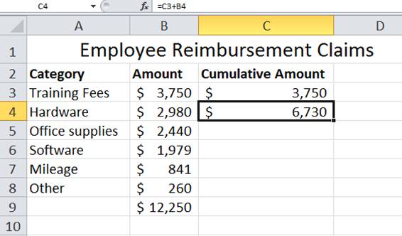
4. Create a column Cumulative Amount (cumulative amount). Let’s start with the first value $ 3750 in the cell B3. Each value is based on the value of the previous cell. In a cell C4 type =C3+B4 and press Enter.
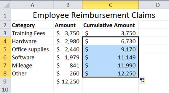
5. To automatically fill in the remaining cells in a column, double-click the autofill handle.
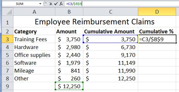
6. Next, create a column Cumulative % (cumulative percentage). To fill this column, you can use the sum of the range Amount and values ​​from column Cumulative Amount. In the formula bar for a cell D3 enter =C3/$B$9 and press Enter. Symbol $ creates an absolute reference such that the sum value (cell reference B9) does not change when you copy the formula down.
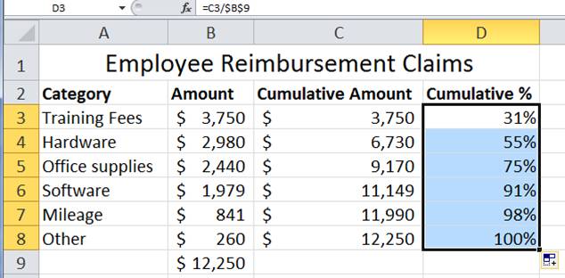
7. Double-click the autofill marker to fill the column with a formula, or click the marker and drag it across the data column.
8. Now everything is ready to start building the Pareto chart!

Part Two: Building a Pareto Chart in Excel

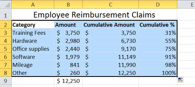
1. Select the data (in our example, cells from A2 by D8).
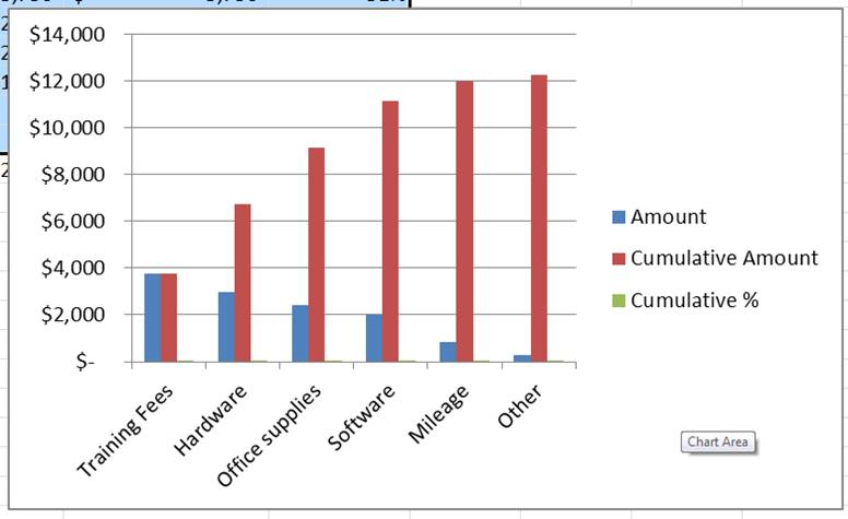
2. Press Alt + F1 on the keyboard to automatically create a chart from the selected data.
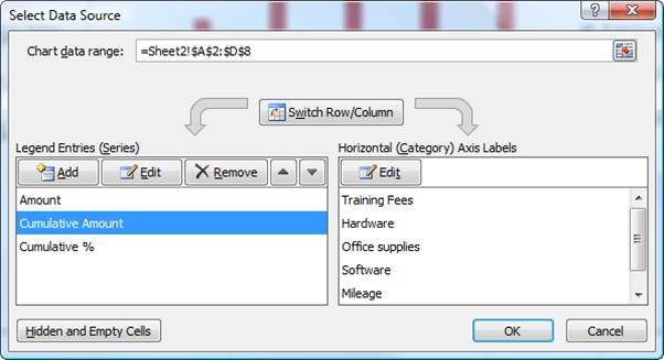
3. Right-click in the chart area and from the menu that appears, click Select data (Select Data). A dialog box will appear Selecting a data source (Select Data Source). Select line Cumulative Amount and press Remove (Remove). Then OK.
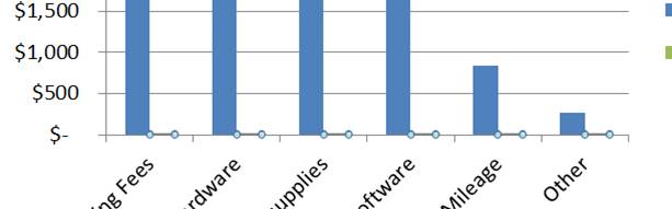
4. Click on the graph and use the arrow keys on your keyboard to move between its elements. When a row of data is selected Cumulative %, which now coincides with the category axis (horizontal axis), right-click on it and select Change the chart type for a series (Change Chart Series Type). Now this series of data is difficult to see, but possible.
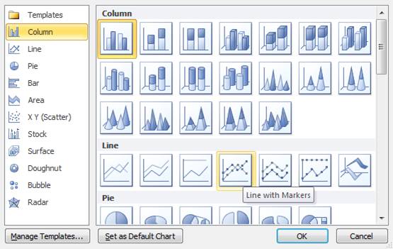
5. A dialog box will appear Change the chart type (Change Chart Type), select line chart.
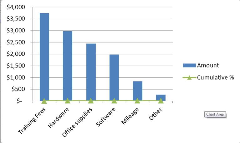
6. So, we got a histogram and a flat line graph along the horizontal axis. In order to show the relief of a line graph, we need another vertical axis.
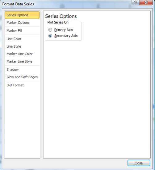
7. Right click on a row Cumulative % and in the menu that appears, click Data series format (Format Data Series). The dialog box of the same name will appear.
8. In section Row Options (Series Options) select Minor Axis (Secondary Axis) and press the button Close (Close).
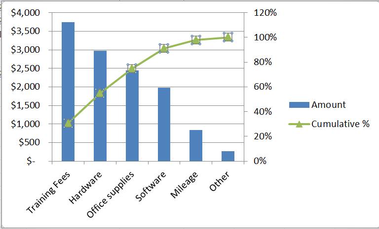
9. The percentage axis will appear, and the chart will turn into a full-fledged Pareto chart! Now we can draw conclusions: the bulk of the costs are tuition fees (Training Fees), equipment (Hardware) and stationery (Office supplies).

With step-by-step instructions for setting up and creating a Pareto chart in Excel at hand, try it out in practice. By applying Pareto analysis, you can identify the most significant problems and take a significant step towards solving them.