


Contents
We have two tables (for example, the old and new versions of the price list), which we need to compare and quickly find the differences:

It is immediately clear that something has been added to the new price list (dates, garlic …), something has disappeared (blackberries, raspberries …), prices have changed for some goods (figs, melons …). You need to quickly find and display all these changes.
For any task in Excel, there is almost always more than one solution (usually 4-5). For our problem, many different approaches can be used:
- function VPR (VLOOKUP) — look for product names from the new price list in the old one and display the old price next to the new one, and then catch the differences
- merge two lists into one and then build a pivot table based on it, where the differences will be clearly visible
- use the Power Query Add-in for Excel
Let’s take them all in order.
Method 1. Comparing tables with the VLOOKUP function
If you are completely unfamiliar with this wonderful feature, then first look here and read or watch a video tutorial on it – save yourself a couple of years of life.
Typically, this function is used to pull data from one table to another by matching some common parameter. In this case, we’ll use it to push the old prices into the new price:

Those products, against which the #N/A error turned out, are not in the old list, i.e. were added. Price changes are also clearly visible.
Pros this method: simple and clear, “classic of the genre”, as they say. Works in any version of Excel.
Cons is also there. To search for products added to the new price list, you will have to do the same procedure in the opposite direction, i.e. pull up new prices to the old price with the help of VLOOKUP. If the sizes of the tables change tomorrow, then the formulas will have to be adjusted. Well, and on really large tables (> 100 thousand rows), all this happiness will decently slow down.
Method 2: Comparing tables using a pivot
Let’s copy our tables one under the other, adding a column with the name of the price list, so that later you can understand from which list which row:

Now, based on the created table, we will create a summary through Insert – PivotTable (Insert — Pivot Table). Let’s throw a field Product to the area of lines, field Price to column area and field Цena into the range:

As you can see, the pivot table will automatically generate a general list of all products from the old and new price lists (no repetitions!) and sort the products alphabetically. You can clearly see the added products (they do not have the old price), the removed products (they do not have the new price) and price changes, if any.
Grand totals in such a table do not make sense, and they can be disabled on the tab Constructor – Grand totals – Disable for rows and columns (Design — Grand Totals).
If prices change (but not the quantity of goods!), then it is enough to simply update the created summary by right-clicking on it – Refresh.
Pros: This approach is an order of magnitude faster with large tables than VLOOKUP.
Cons: you need to manually copy the data under each other and add a column with the name of the price list. If the sizes of the tables change, then you have to do everything all over again.
Method 3: Comparing tables with Power Query
Power Query is a free add-in for Microsoft Excel that allows you to load data into Excel from almost any source and then transform this data in any desired way. In Excel 2016, this add-in is already built in by default on the tab Data (Data), and for Excel 2010-2013 you need to download it separately from the Microsoft website and install it – get a new tab Power Query.
Before loading our price lists into Power Query, they must first be converted into smart tables. To do this, select the range with data and press the combination on the keyboard Ctrl+T or select the tab on the ribbon Home – Format as a table (Home — Format as Table). The names of the created tables can be corrected on the tab Constructor (I will leave the standard Table 1 и Table 2, which are obtained by default).
Load the old price in Power Query using the button From Table/Range (From Table/Range) from the tab Data (Date) or from the tab Power Query (depending on the version of Excel). After loading, we will return back to Excel from Power Query with the command Close and load – Close and load in… (Close & Load — Close & Load To…):

… and in the window that appears then select Just create a connection (Connection Only).
Repeat the same with the new price list.
Now let’s create a third query that will combine and compare the data from the previous two. To do this, select in Excel on the tab Data – Get Data – Combine Requests – Combine (Data — Get Data — Merge Queries — Merge) or press the button Combine (Merge) tab Power Query.
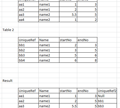
In the join window, select our tables in the drop-down lists, select the columns with the names of the goods in them, and at the bottom, set the join method – Complete external (Full Outer):

After clicking on OK a table of three columns should appear, where in the third column you need to expand the contents of nested tables using the double arrow in the header:

As a result, we get the merging of data from both tables:

It is better, of course, to rename the column names in the header by double-clicking on more understandable ones:

And now the most interesting. Go to tab Add column (Add Column) and click on the button Conditional column (Conditional Column). And then in the window that opens, enter several test conditions with their corresponding output values:

It remains to click on OK and upload the resulting report to Excel using the same button close and download (Close & Load) tab Home (Home):

Beauty.
Moreover, if any changes occur in the price lists in the future (lines are added or deleted, prices change, etc.), then it will be enough just to update our requests with a keyboard shortcut Ctrl+Alt+F5 or by button Refresh all (Refresh All) tab Data (Date).
Pros: Perhaps the most beautiful and convenient way of all. Works smartly with large tables. Does not require manual edits when resizing tables.
Cons: Requires the Power Query add-in (in Excel 2010-2013) or Excel 2016 to be installed. The column names in the source data must not be changed, otherwise we will get the error “Column such and such was not found!” when trying to update the query.
- How to collect data from all Excel files in a given folder using Power Query
- How to find matches between two lists in Excel
- Merging two lists without duplicates