All about creating a chart in Excel. Step by step guide with screenshots

Excel is an amazing program that allows you to process not only numerical data. With its help, you can visually represent any information by building diagrams of varying degrees of complexity. It is enough just to specify the data in the cells, and the program will automatically build a chart based on them. Say it’s amazing!

In this case, the user can customize the appearance of the chart that he likes. Today we will analyze in detail the available charting tools in Excel and other similar programs. After all, the basic principle is not limited to only the office suite from Microsoft, right? Therefore, the principles described here may well be used when working with other spreadsheet programs such as LibreOffice, WPS Office, or Google Sheets.

Building a chart based on Excel spreadsheet data

Before proceeding directly to building Excel charts, you need to understand what it is and what they are for. There are several ways to present information:

1. Auditory.
2. Text.
3. Visual.
4. Interactive.

The most familiar to the average person is the auditory and textual way of transmitting information. The first involves the use of voice in order to present certain data, facts and figures. A very unreliable method that is not able to deliver information perfectly. The only thing it can be used for during presentations is to evoke certain emotions in the audience. Text can convey text, but has a much lower ability to evoke certain emotions. The interactive method involves the involvement of the audience (for example, investors). But if we talk about business data, then you can’t play much here.

The visual way of presenting information opens up a huge number of advantages. It helps to combine all the advantages of the remaining methods. It transmits information very accurately, since it contains all the numbers, and a person can analyze the data based on the graph. He is able to evoke emotions. For example, just look at the graph of the spread of coronavirus infection in recent times, and it immediately becomes clear how the graph can easily affect the emotional part of the brain.

And what is important, it is able to involve a person who can selectively look at one or another part of the chart and analyze the information that he really needs. This is why charts have become so widespread around the world. They are used in various fields of human activity:

1. During the presentation of the results of research at various levels. This is a universal point for both students and scientists defending a dissertation. This type of presentation of information, like a diagram, makes it possible to pack a large amount of information into a very convenient form and present all this data to a wide audience so that it immediately becomes clear. The diagram allows you to inspire confidence in what an applicant for a master’s or doctoral degree says.
2. During business presentations. Especially the creation of diagrams is necessary if it is necessary to present the project to the investor or report on the progress of its work.

   This will make it clear that the authors of the project themselves take it seriously. Among other things, investors will be able to analyze all the necessary information on their own. Well, the point about the fact that the presence of diagrams in itself inspires confidence, because it is associated with the accuracy of the presentation of information, remains both for this area and all the following ones.

3. For reporting to superiors. Management loves the language of numbers. Moreover, the higher it is in rank, the more important it is for him. The owner of any business needs to understand how much this or that investment pays off, which sectors of production are unprofitable and which are profitable, and understand many other important aspects.

There are many other areas in which charts can be used. For example, in teaching. But no matter for what specific purposes they are compiled, if they are done in Excel, then in fact almost nothing needs to be done. The program will do everything for the person himself. In fact, building charts in Excel is not fundamentally different from creating regular tables. Therefore, anyone can create them very simply. But for clarity, let’s describe the basic principle in the form of instructions. Follow these steps:

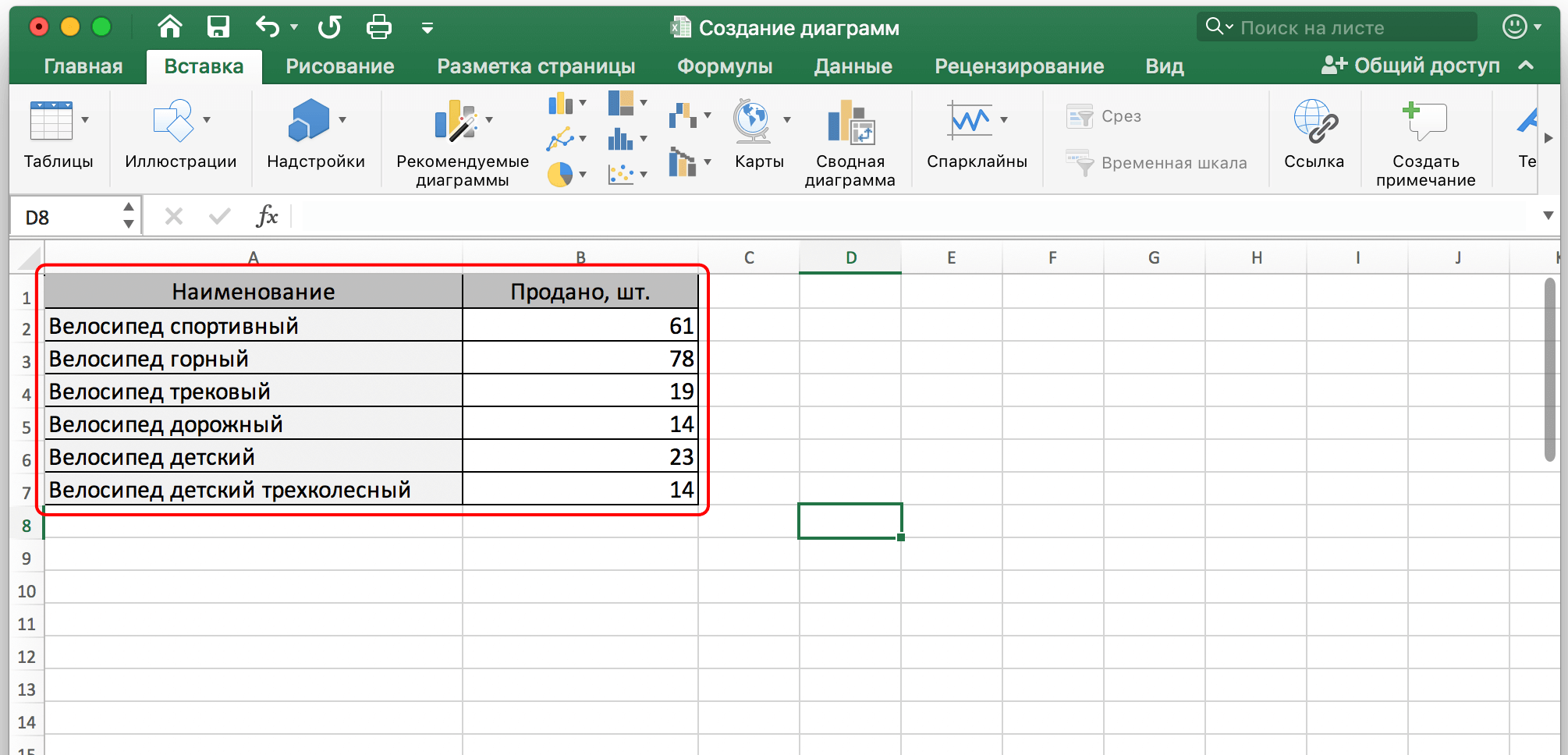
1. Before creating a graph or chart, you must first create a table with the information that will be used for this. Let’s also create such a table.
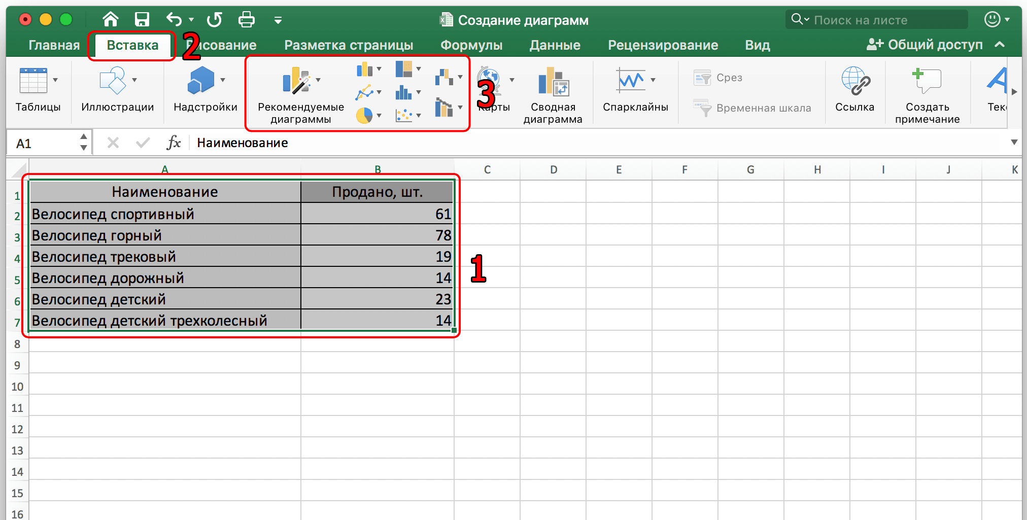
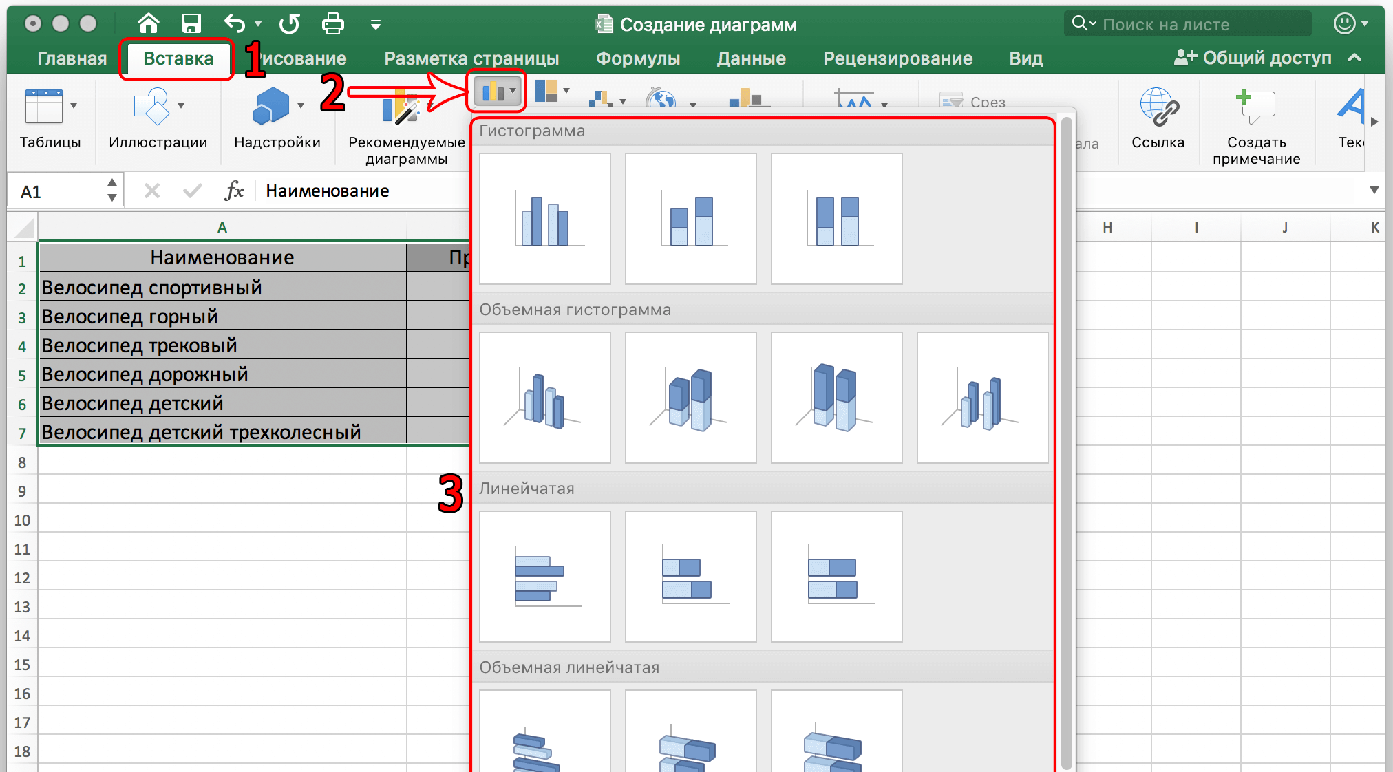
2. After creating the table, you need to find the area that will be used for the basis of the chart, and then click on the “Insert” tab with the left mouse button once. After that, the user will be able to choose the type of chart that he likes. This is a graph, and a pie chart, and a histogram. There is room to expand.
   

   Attention! Programs differ among themselves in the number of types of diagrams that can be created.

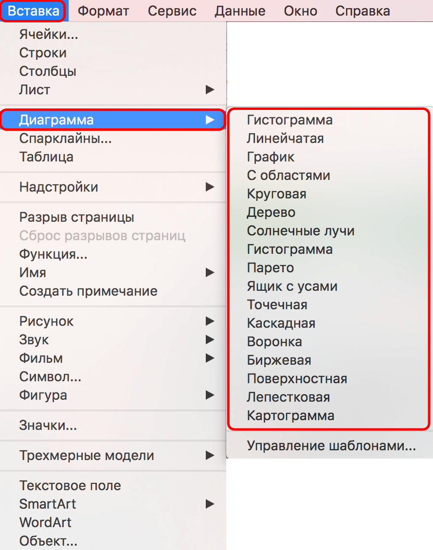
3. You can use many other types of charts. They just aren’t that popular. To view the entire list of available types, go to the “Diagram” menu and select a specific type there. We see that there is a slightly different menu here. There is nothing strange about this, since the buttons themselves may differ not only depending on the version of the office suite, but also on the very variety of the program and operating system. Here it is important to understand the logic first, and everything else should become intuitive.
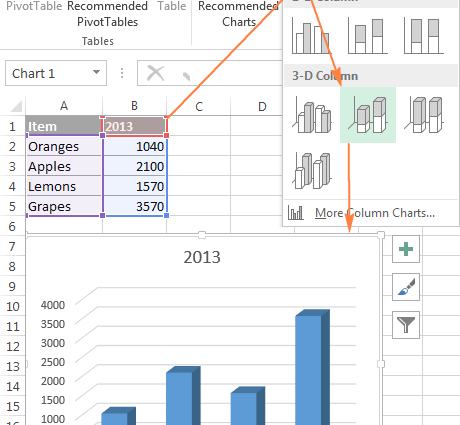
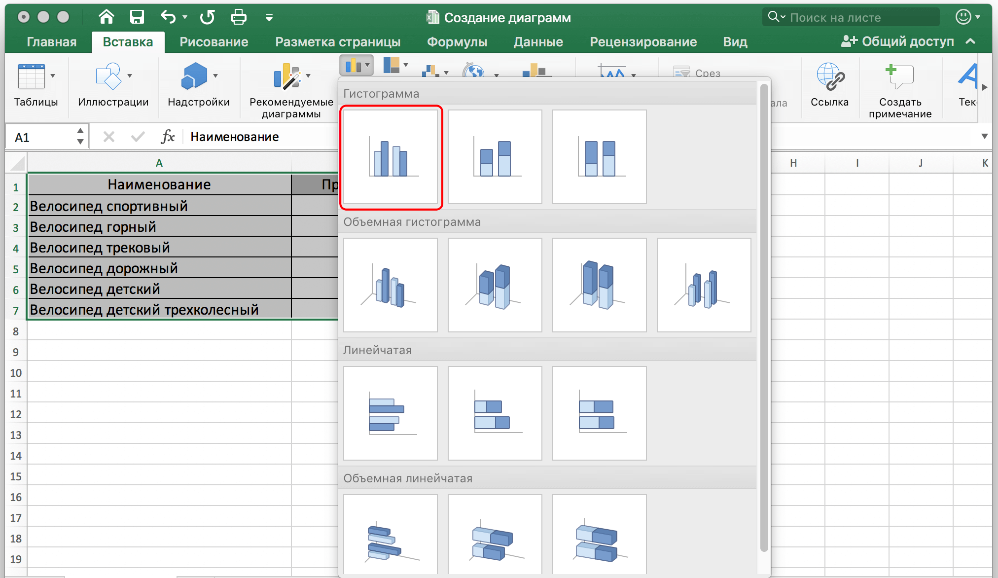
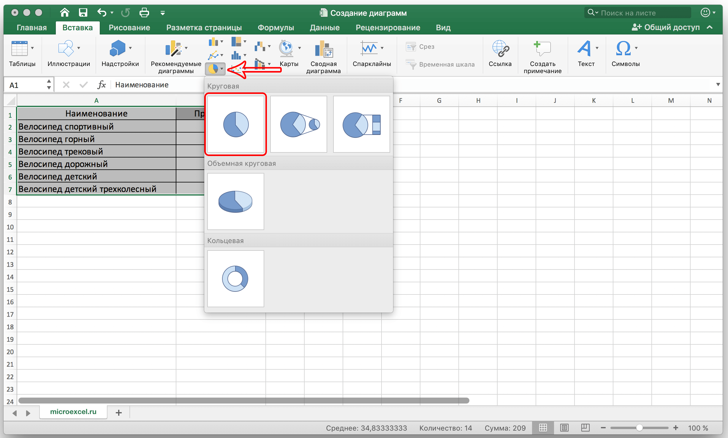
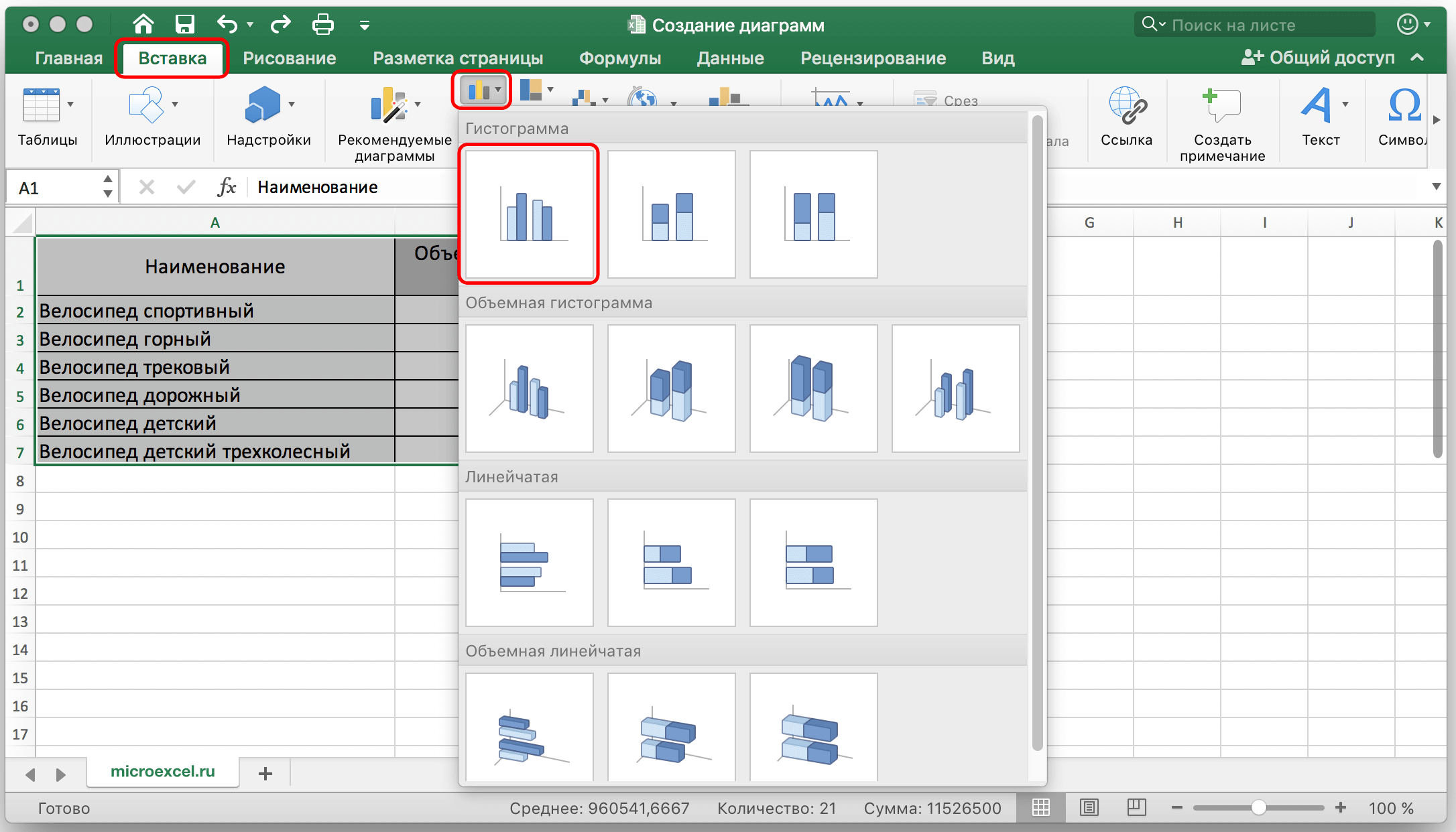
4. After selecting the appropriate chart type, click on it. You will then be presented with a list of subtypes, and you will need to select the one that best suits your situation. For example, if a histogram was selected, then you can select regular, bar, volume, and so on. The list of types with pictures, by which you can understand how the final diagram will look, is located directly in this menu.
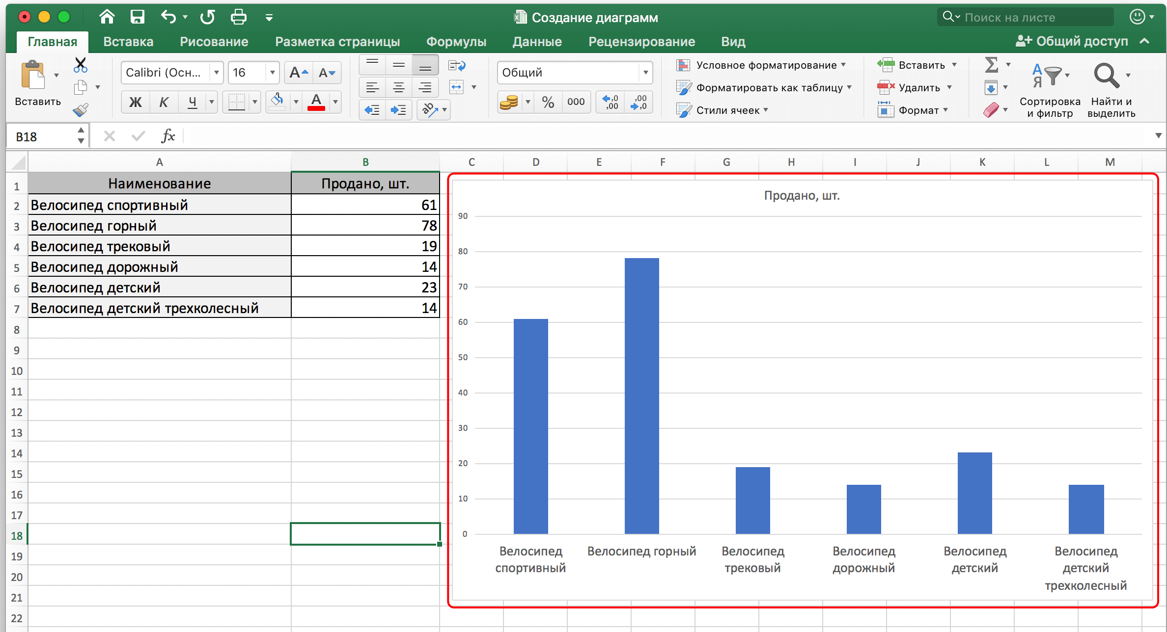
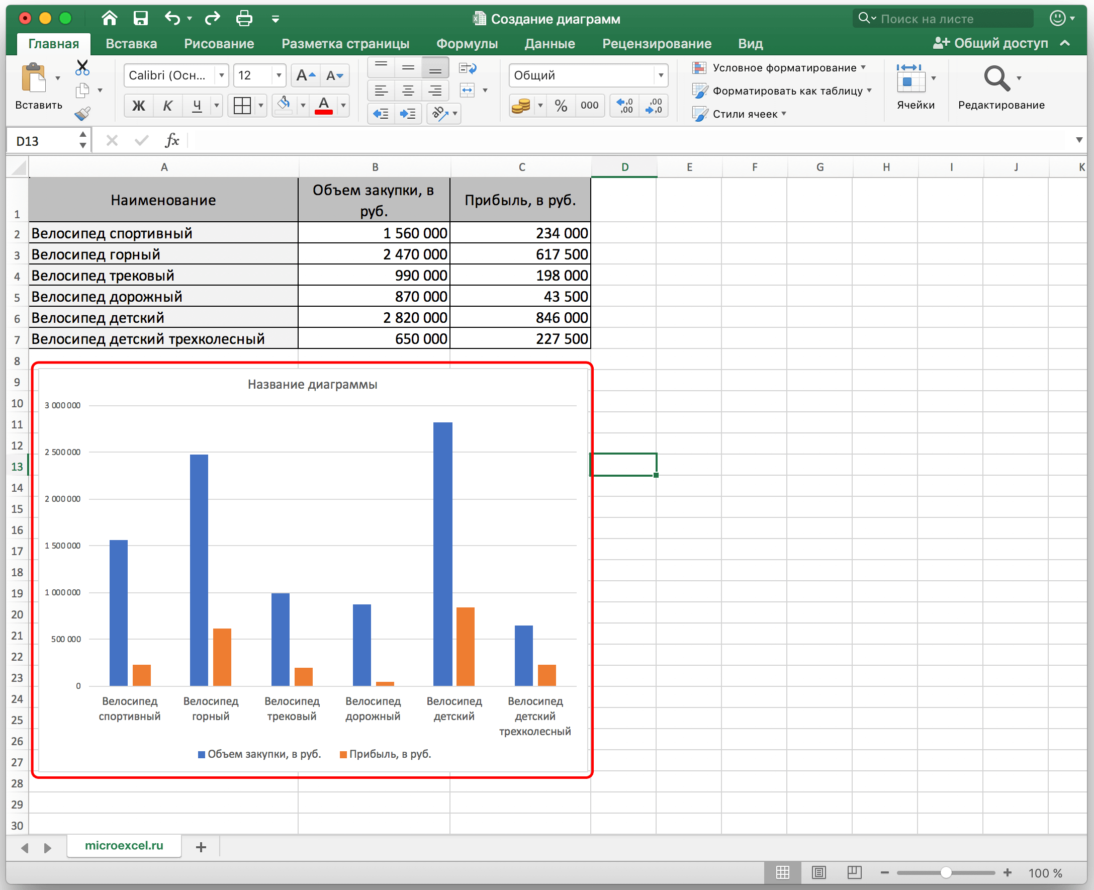
5. We click on the subtype that we are interested in, after which the program will do everything automatically. The resulting chart will appear on the screen.
6. In our case, the picture turned out as follows.
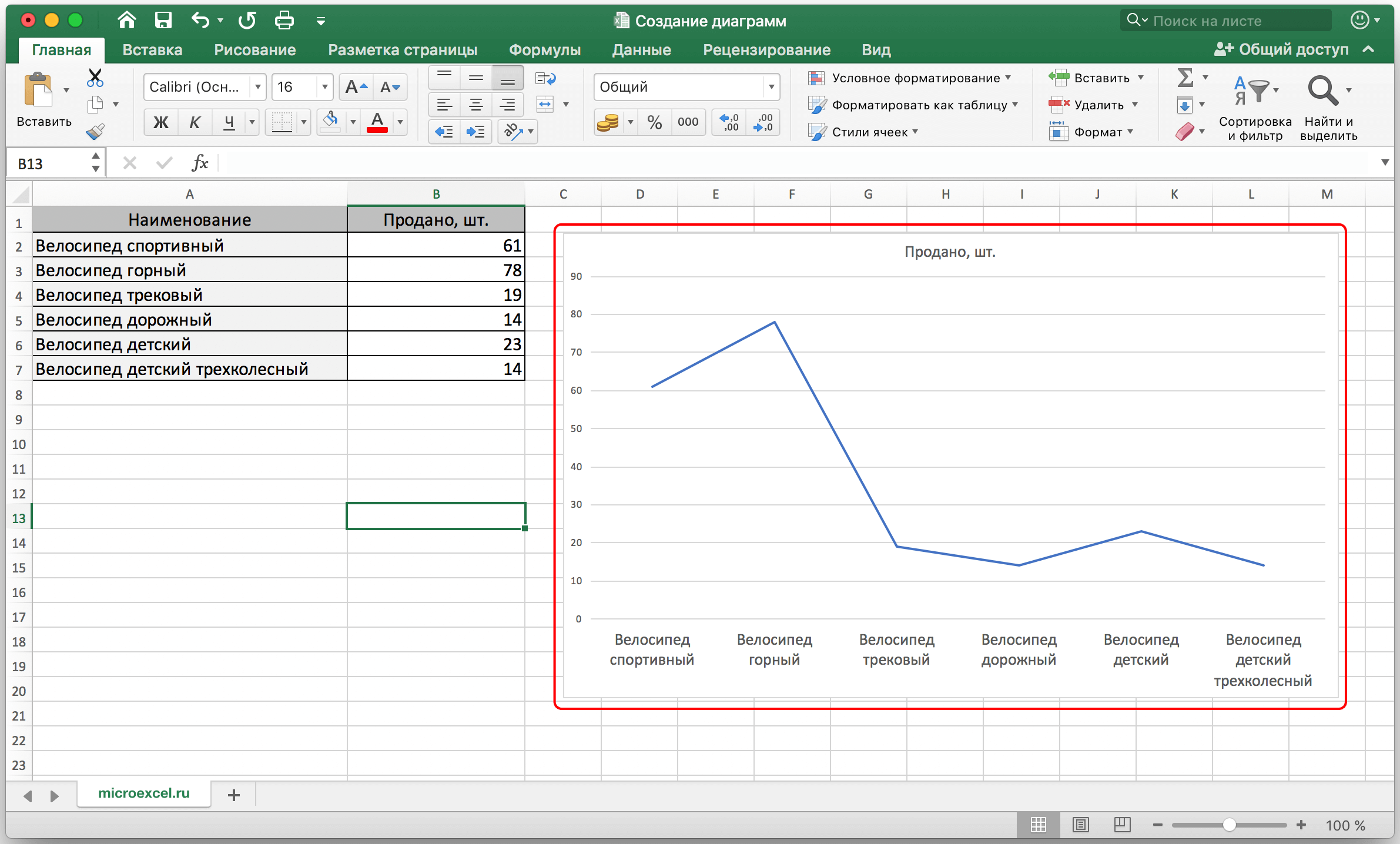
7. If we chose the “Chart” type, then our chart would look like this.
8. The pie chart has the following form.

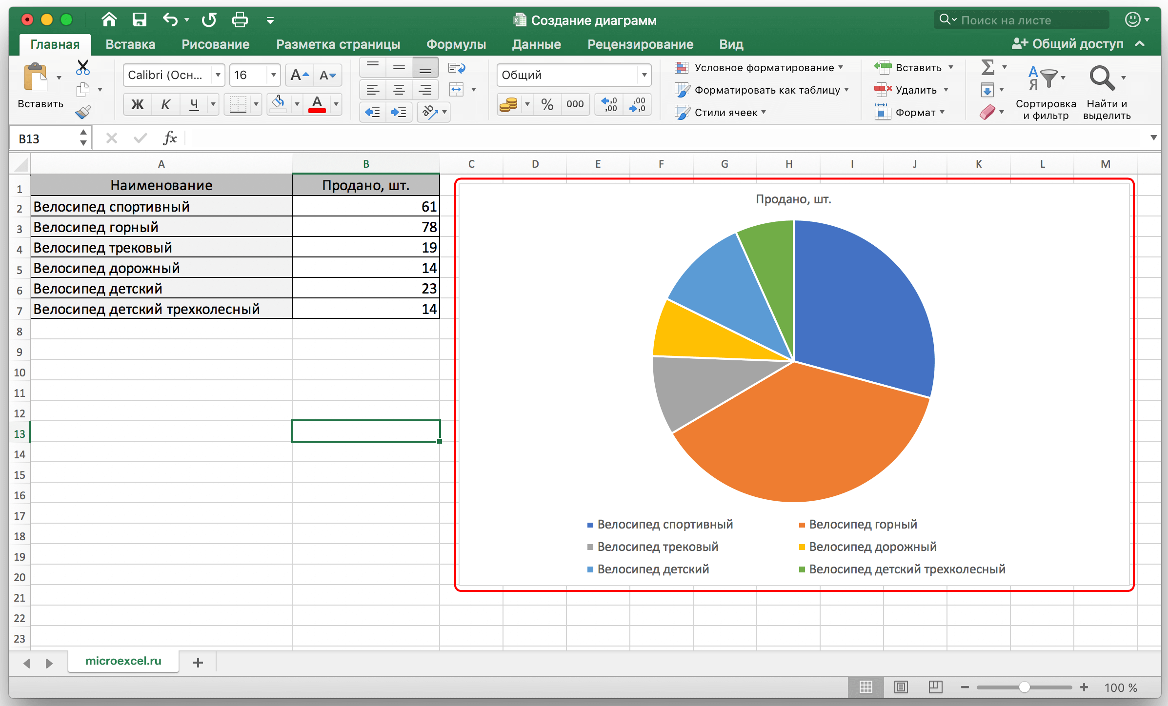
As you can see, the instructions are not complicated at all. It is enough to enter a little data, and the computer will do the rest for you.

How to work with charts in Excel

After we have made the chart, we can already customize it. To do this, you need to find the “Designer” tab at the top of the program. This panel has the ability to set various properties of the chart we created earlier. For example, the user can change the color of the columns, as well as make more fundamental changes. For example, change the type or subtype. So, to do this, you need to go to the “Change chart type” item, and in the list that appears, you can select the desired type. Here you can also see all available types and subtypes.

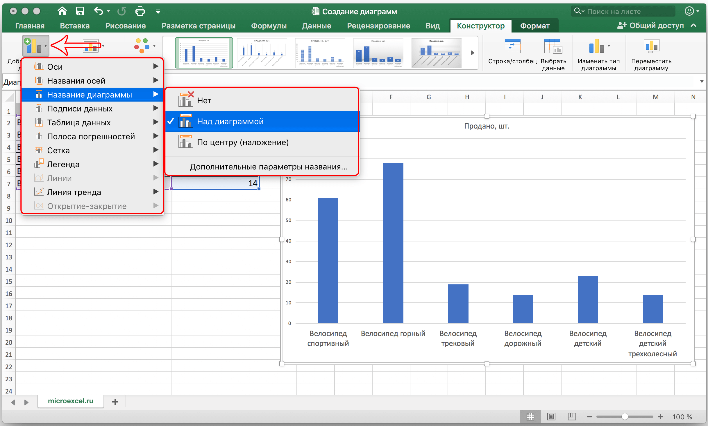
We can also add some element to the created chart. To do this, click on the appropriate button, which is located immediately on the left side of the panel.

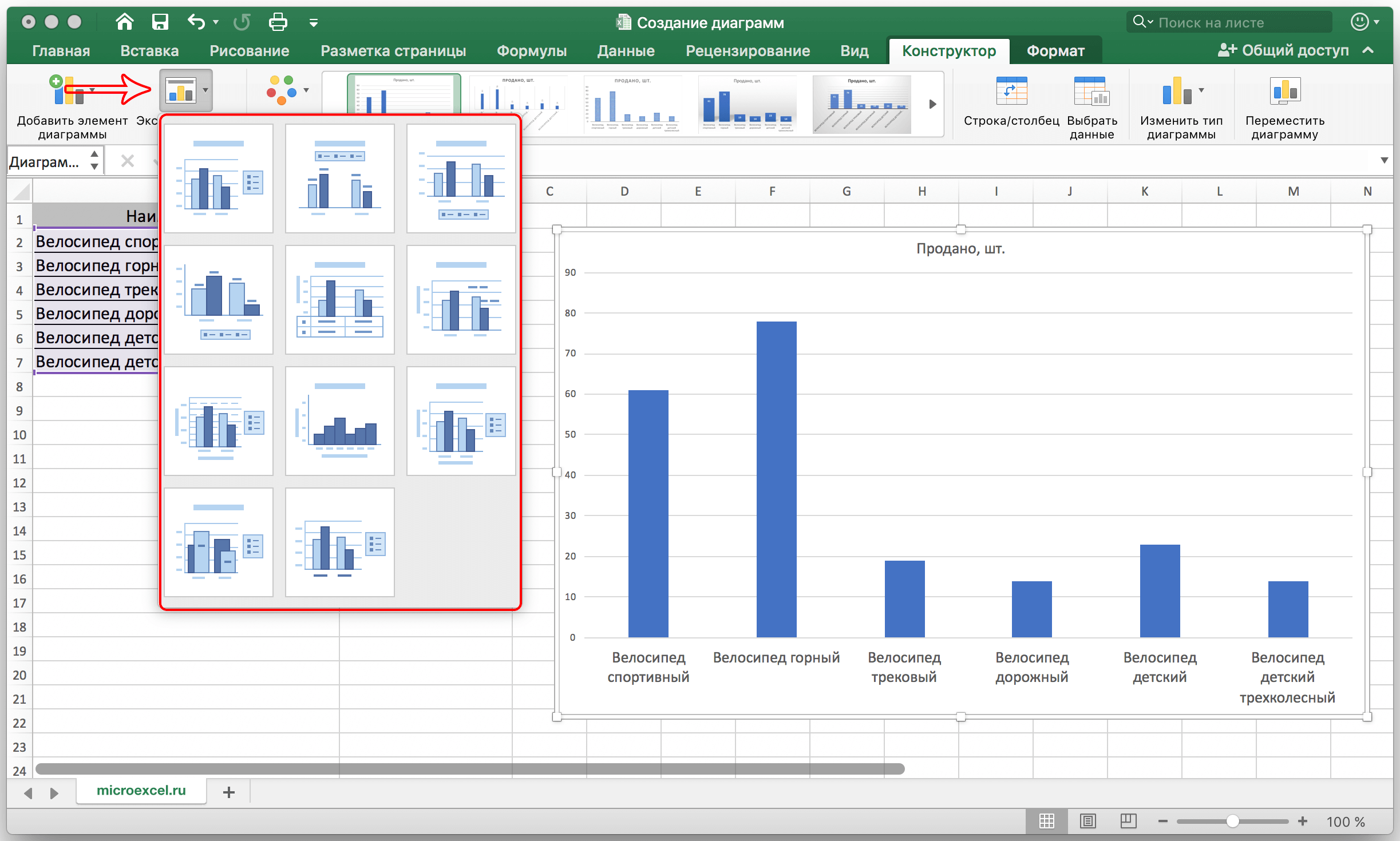
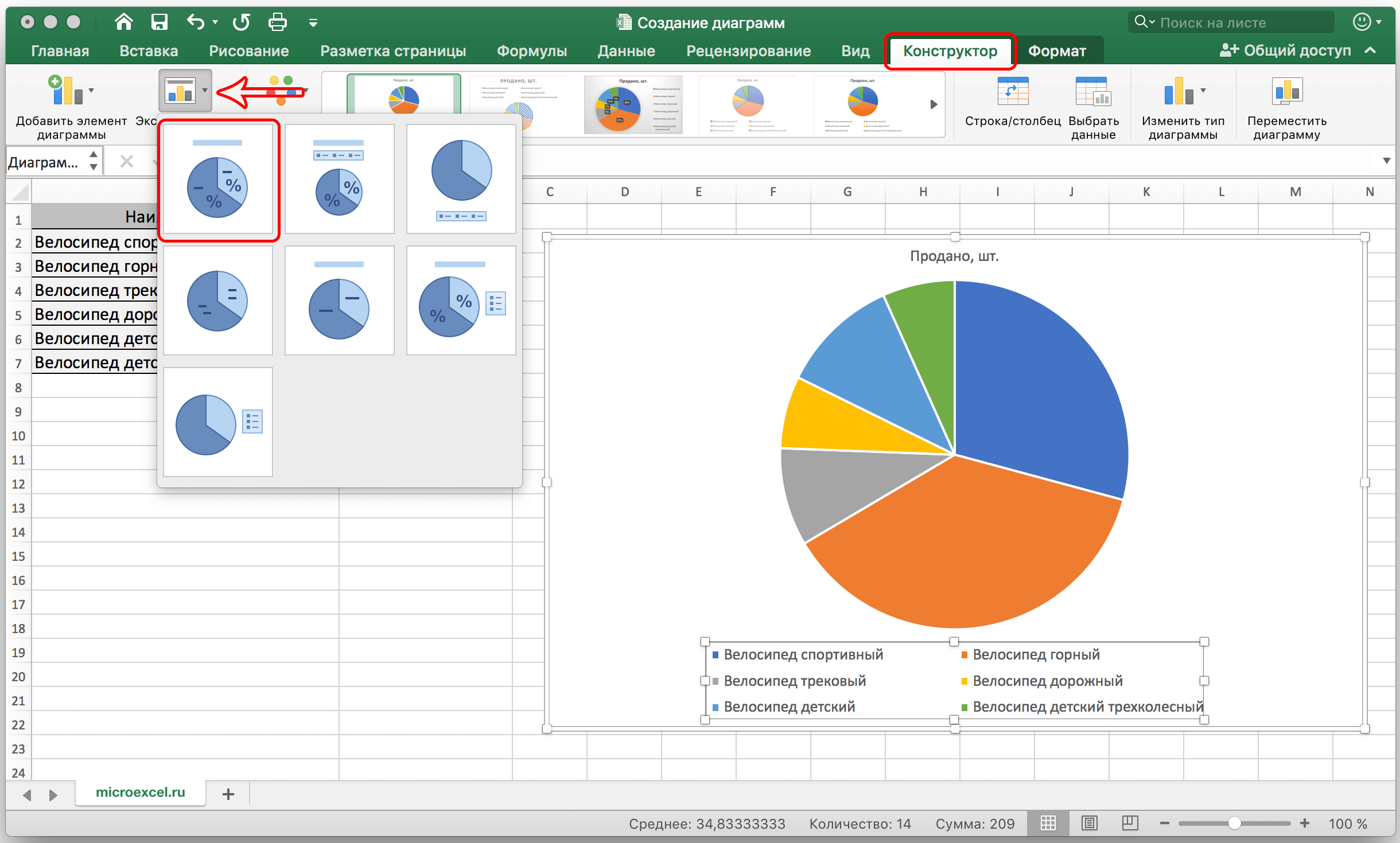
You can also do a quick setup. There is a special tool for this. The button corresponding to it can be found to the right of the “Add Chart Element” menu. Here you can choose almost any design option that fits the current task.

It is also quite useful if there is a designation of each of them near the columns. To do this, you need to add captions through the “Add Chart Element” menu. After clicking on this button, a list will open in which we are interested in the corresponding item. Then we choose how the caption will be displayed. In our example – indicated in the screenshot.

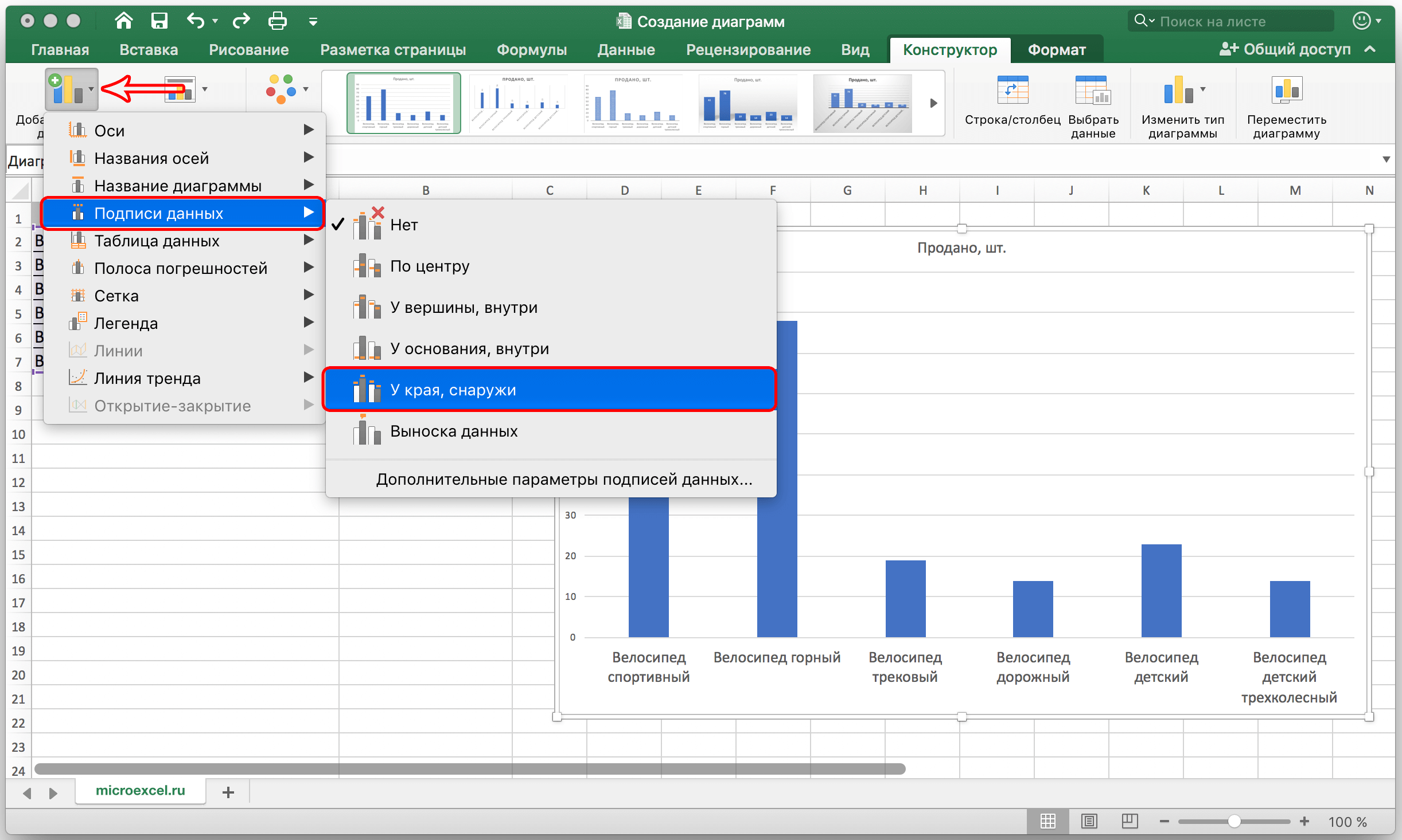
Now this chart not only clearly shows the information, but it can also be used to understand what exactly each column means.

How to set up a chart with percentages?

Now let’s move on to specific examples. If we need to create a chart in which we work with percentages, then we need to select a circular type. The instruction itself is as follows:

1. According to the mechanism described above, it is necessary to create a table with data and select a range with data that will be used to build a chart. After that, go to the “Insert” tab and select the appropriate type.
2. After the previous step is completed, the program will open the “Constructor” tab automatically. Next, the user needs to analyze the available options and find the one where the percent icons are displayed.
3. Further work with a pie chart will be carried out in a similar way.

How to change font size in excel chart

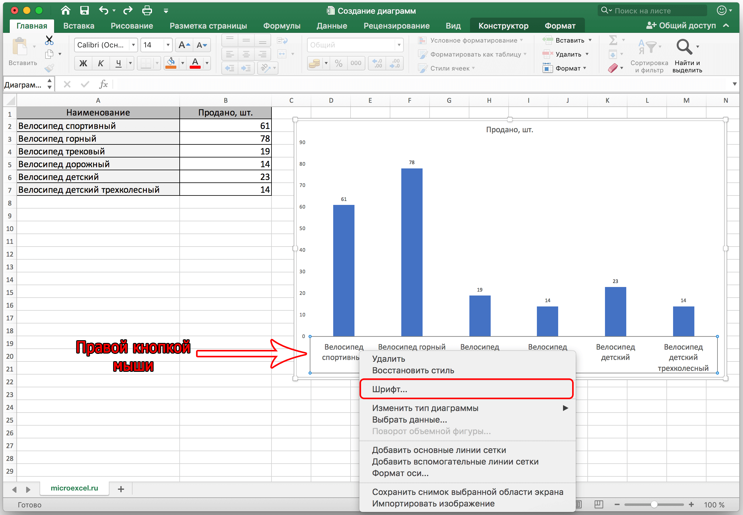
Customizing chart fonts allows you to make it much more flexible and informative. It is also useful if it needs to be shown on a big screen. Often the standard size is not enough to be visible to people from the back row. To set the chart font sizes, you need to right-click on the appropriate label and click on the font item in the list that appears.

After that, you need to make all the necessary adjustments and click on the “OK” button to save them.

Pareto chart – definition and construction principle in Excel

Many people know the Pareto principle, which says that 20% of effort gives 80% of the result and vice versa. Using this principle, you can draw a diagram that will allow you to most find the most effective actions from which the result was the largest. And to build a chart of this type, the built-in tools of Microsoft Excel are enough. To build such an infographic, you must select the “Histogram” type. The sequence of our actions is as follows:

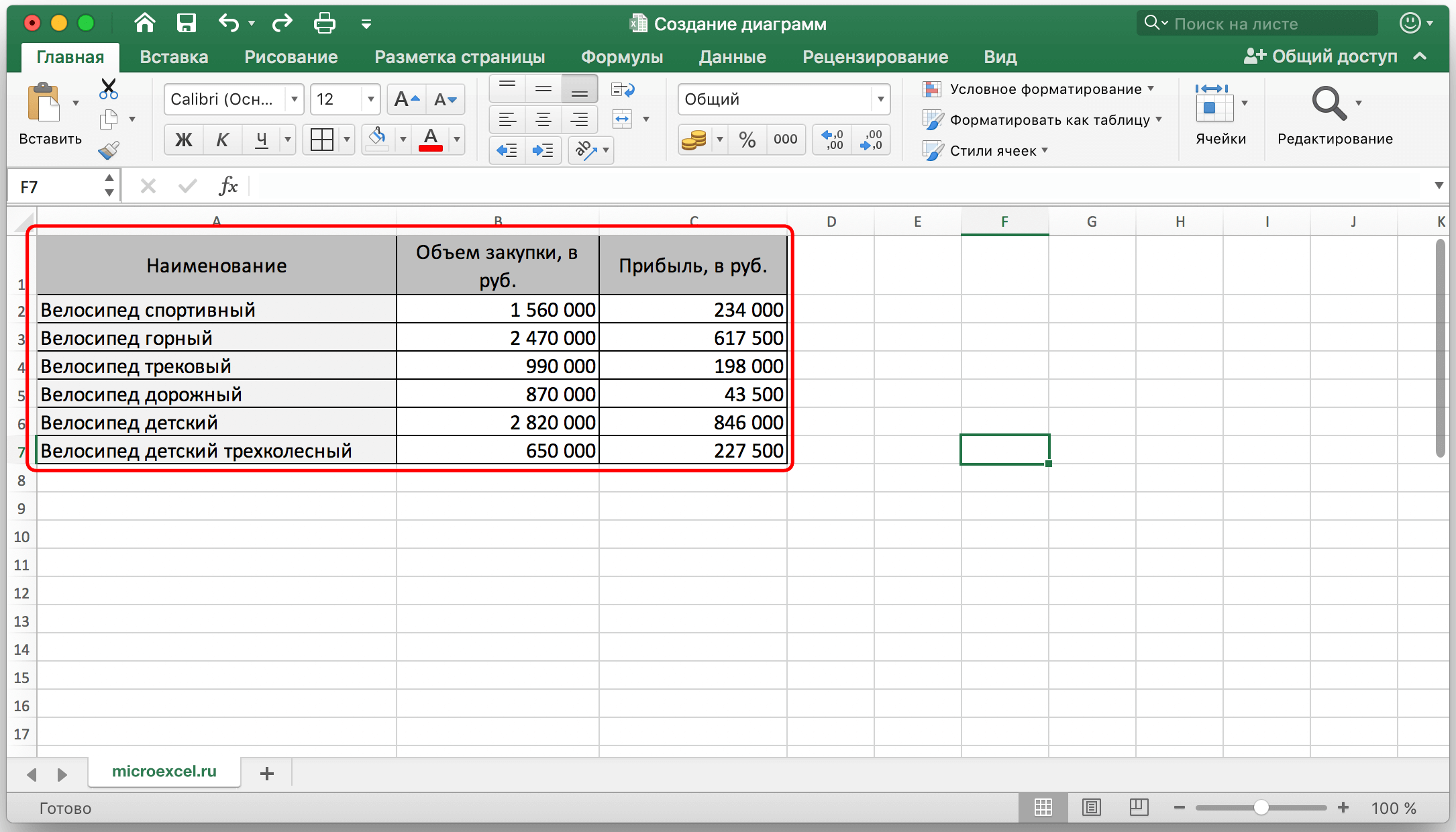
1. Let’s generate a table that describes the names of the products. We will have multiple columns. The first column will describe the total amount of the purchase of goods in money. The second column records the profit from the sale of these goods.
2. We make the most ordinary histogram. To do this, you need to find the “Insert” tab, and then select the appropriate chart type.
3. Now we have a chart ready, which has 2 columns of different colors, each of which represents a specific column. Below you can see the legend of the chart, according to which we understand where which column is.
4. The next step that we need to perform is editing the column that is responsible for the profit. We are faced with the task of seeing its change in dynamics. Therefore, we need a “Graph” chart type. Therefore, in the “Designer” tab, we need to find the “Change Chart Type” button and click on it. Then select a schedule from the list. It is important not to forget to select the appropriate column before doing this.

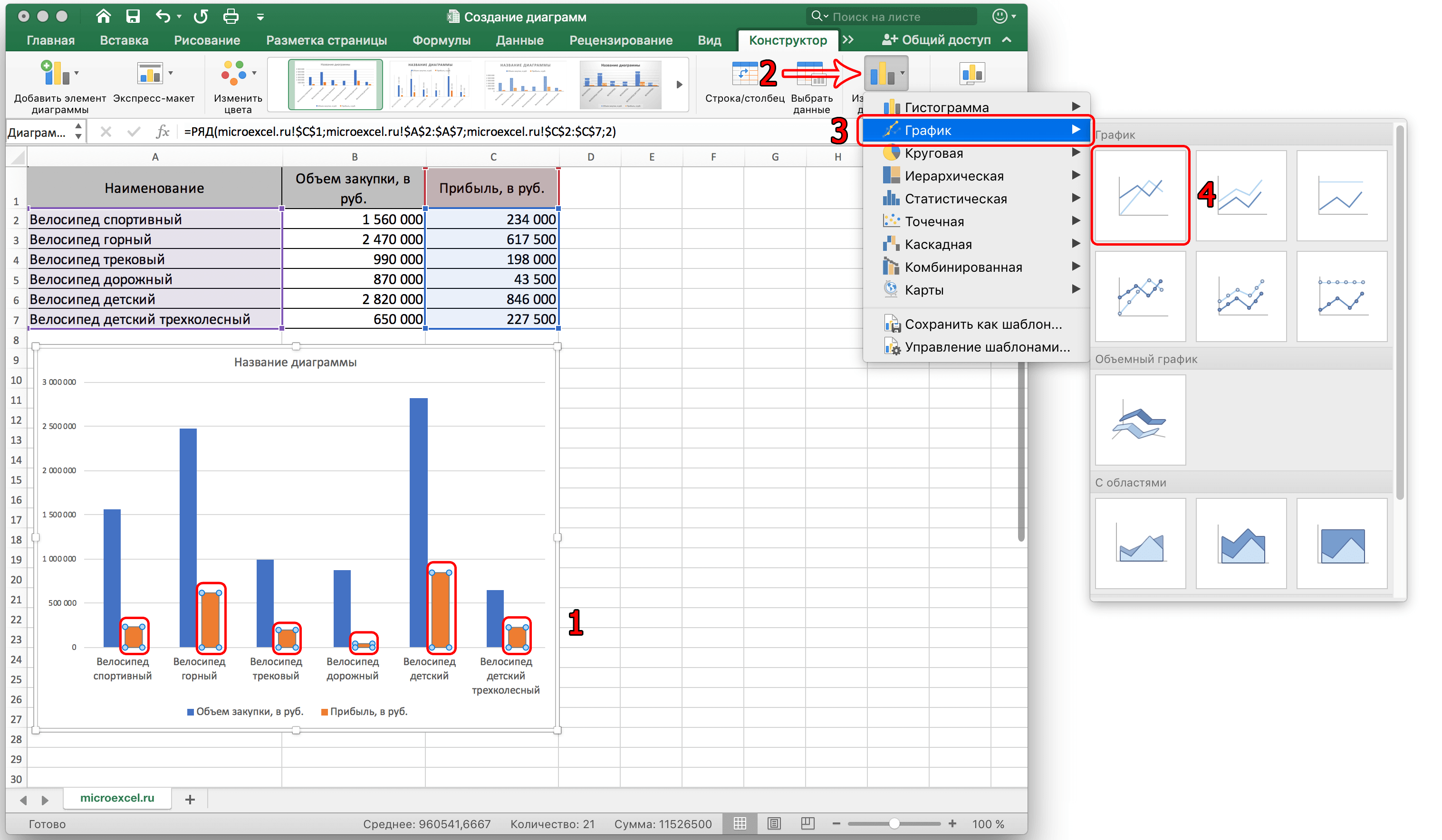
Now the Pareto chart is ready. You can analyze the effectiveness and determine what can be sacrificed without fear. Editing this chart is done in exactly the same way as before. For example, you can add labels to bars and points on a chart, change the color of lines, columns, and so on.

Thus, Excel has a huge toolkit for creating charts and customizing them. If you experiment with the settings yourself, a lot becomes clear and you will be able to create graphs of any complexity and make them readable. And this is exactly what any investor, boss or client needs. Diagrams find their application in all possible fields of activity. Therefore, Excel is considered the main program in order to make money. Now you have come even closer to them. Good luck.