Contents
Yesterday in the marathon 30 Excel functions in 30 days we had fun with the function REPT (REPEAT) by creating charts inside a cell and using it for simple counting. It’s Monday, and once again it’s time for us to put on our thinker hats.
On the 16th day of the marathon, we will study the function LOOKUP (VIEW). This is a close friend VLOOKUP (VLOOKUP) and HLOOKUP (GPR), but it works a little differently.
So, let’s study the theory and test the function in practice LOOKUP (VIEW). If you have additional information or examples on how to use this feature, please share them in the comments.
Function 16: LOOKUP
Function LOOKUP (LOOKUP) returns a value from one row, one column, or from an array.
How can I use the LOOKUP function?
Function LOOKUP (LOOKUP) returns the result, depending on the value you are looking for. With its help you will be able to:
- Find the last value in a column.
- Find the last month with negative sales.
- Convert student achievement from percentages to letter grades.
Syntax LOOKUP
Function LOOKUP (LOOKUP) has two syntactic forms – vector and array. In vector form, the function looks for the value in the given column or row, and in array form, it looks for the value in the first row or column of the array.
The vector form has the following syntax:
LOOKUP(lookup_value,lookup_vector,result_vector)
ПРОСМОТР(искомое_значение;просматриваемый_вектор;вектор_результатов)
- lookup_value (lookup_value) – Can be text, number, boolean, name, or link.
- lookup_vector (lookup_vector) – A range consisting of one row or one column.
- result_vector (result_vector) – a range consisting of one row or one column.
- argument ranges lookup_vector (lookup_vector) and result_vector (result_vector) must be the same size.
The array form has the following syntax:
LOOKUP(lookup_value,array)
ПРОСМОТР(искомое_значение;массив)
- lookup_value (lookup_value) – Can be text, number, boolean, name, or link.
- the search is performed according to the dimension of the array:
- if the array has more columns than rows, then the search occurs in the first row;
- if the number of rows and columns is the same or there are more rows, then the search occurs in the first column.
- the function returns the last value from the found row/column.
Traps LOOKUP (VIEW)
- In function LOOKUP (BROWSE) there is no option to search for an exact match, which is in VLOOKUP (VLOOKUP) and in HLOOKUP (GPR). If there is no search value, then the function will return the maximum value not exceeding the search value.
- The array or vector being searched must be sorted in ascending order, otherwise the function may return an incorrect result.
- If the first value in the array/vector being looked up is greater than the lookup value, then the function will generate an error message #AT (#N/A).
Example 1: Finding the last value in a column
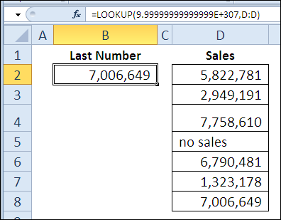
In the form of an array function LOOKUP (LOOKUP) can be used to find the last value in a column.
Excel help quotes value 9,99999999999999E + 307 as the largest number that can be written in a cell. In our formula, it will be set as the desired value. It is assumed that such a large number will not be found, so the function will return the last value in column D.
In this example, the numbers in column D are allowed not to be sorted, in addition, text values may come across.
=LOOKUP(9.99999999999999E+307,D:D)
=ПРОСМОТР(9,99999999999999E+307;D:D)
Example 2: Find the last month with a negative value
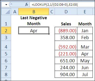
In this example, we will use the vector shape LOOKUP (VIEW). Column D contains the sales values, and column E contains the names of the months. In some months, things didn’t go well, and negative numbers appeared in cells with sales values.
To find the last month with a negative number, the formula with LOOKUP (LOOKUP) will check for each sales value that it is less than 0 (inequality in the formula). Next, we divide 1 on the result, we end up with either 1, or an error message #DIV/0 (#SECTION/0).
Since the desired value is 2 is not found, the function will select the last found 1, and return the corresponding value from column E.
=LOOKUP(2,1/(D2:D8<0),E2:E8)
=ПРОСМОТР(2;1/(D2:D8<0);E2:E8)
Explanation: In this formula, instead of the argument lookup_vector (lookup_vector) expression substituted 1/(D2:D8<0), which forms an array in the computer's RAM, consisting of 1 and error values #DIV/0 (#SECTION/0). 1 indicates that the corresponding cell in the range D2:D8 contains a value less than 0, and the error #DIV/0 (#DIV/0) – what is greater than or equal to 0. As a result, our task is to find the last 1 in the created virtual array, and based on this, return the name of the month from the range E2:E8.
Example 3: Converting student achievement from percentages to letter grades
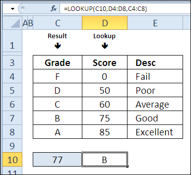
Previously, we have already solved a similar problem using the function VLOOKUP (VPR). Today we will use the function LOOKUP (VIEW) in vector form to convert student achievement from percentages to letter grades. Unlike VLOOKUP (VLOOKUP) for a function LOOKUP (VIEW) It doesn't matter if the percentages are in the first column of the table. You can select absolutely any column.
In the following example, the scores are in column D, sorted in ascending order, and their corresponding letters are in column C, to the left of the column being searched.
=LOOKUP(C10,D4:D8,C4:C8)
=ПРОСМОТР(C10;D4:D8;C4:C8)