


Contents
A huge number of Excel users make the same mistake. They confuse two fundamentally different types of operations: inside the cell and behind it. But the difference between them is huge.
The fact is that each cell is a full-featured element, which is an input field with a lot of possibilities. Formulas, numbers, text, logical operators, and so on are entered there. The text itself can be styled: change its size and style, as well as its location inside the cell.
For example, in this picture you can see that the text inside the cell is red and bold.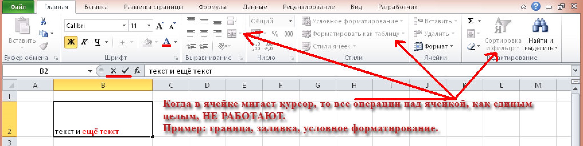
In this case, it is important to pay attention to the fact that the cell shown in the picture is currently in content editing mode. To understand what specific state the cell is in in your case, you can use the text cursor inside. But even if it is not visible, the cell may be in edit mode. You can understand this by the presence of active buttons for confirming and canceling input.
An important feature of this mode is that it is impossible to perform all possible operations with a cell in it. If you look at the ribbon toolbar, you will see that most of the buttons are not active. This is where the main mistake is expressed. But let’s talk about everything in order, starting with the very basics and then we will increase the level of complexity so that everyone can learn something useful.
Basic Concepts
So, the main element of the table is the cell. It is located at the intersection of a column and a row, and therefore it has its own address, which can be used in formulas in order to point to it, get certain data, and so on.
For example, cell B3 has the following coordinates: row 3, column 2. You can see it in the upper left corner, directly below the navigation menu.
The second important concept is the workbook. This is a document opened by the user, which contains a list of sheets, which in turn consist of cells. Any new document initially does not contain any information, and in the corresponding wine field the address of the cell currently selected.
The column and row names are also displayed. When one of the cells is selected, the corresponding elements in the coordinate bar will be highlighted in orange.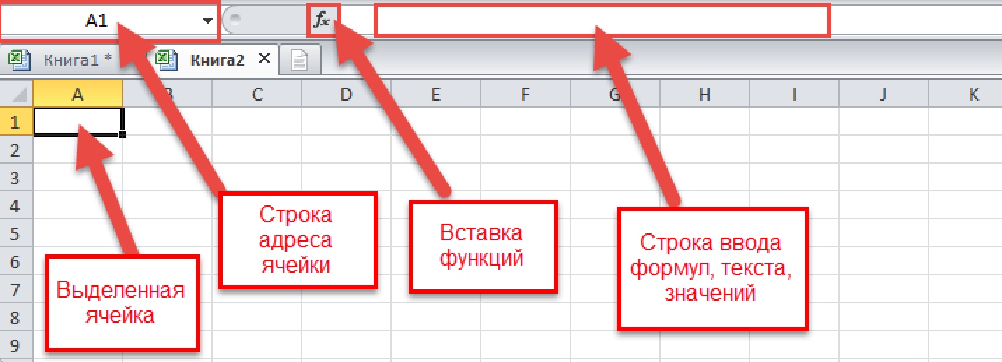
To enter information, it is necessary, as we already understood above, to switch to edit mode. You need to select the appropriate cell by left clicking on it, and then just enter the data. You can also navigate between different cells using the keyboard using the arrow buttons.
Basic Cell Operations
Select cells in one range
Grouping information in Excel is carried out according to a special range. In this case, several cells are selected at once, as well as rows and columns, respectively. If you select them, the entire area is displayed, and the address bar provides a summary of all the selected cells.
Merging cells
Once the cells have been selected, they can now be merged. Before doing this, it is recommended to copy the selected range by pressing the Ctrl + C key combination and move it to another location using the Ctrl + V keys. This way you can save a backup copy of your data. This must be done, because when cells are merged, all the information contained in them is erased. And in order to restore it, you must have a copy of it.
Next, you need to click on the button shown in the screenshot. There are several ways to merge cells. You need to choose the one that best suits the situation.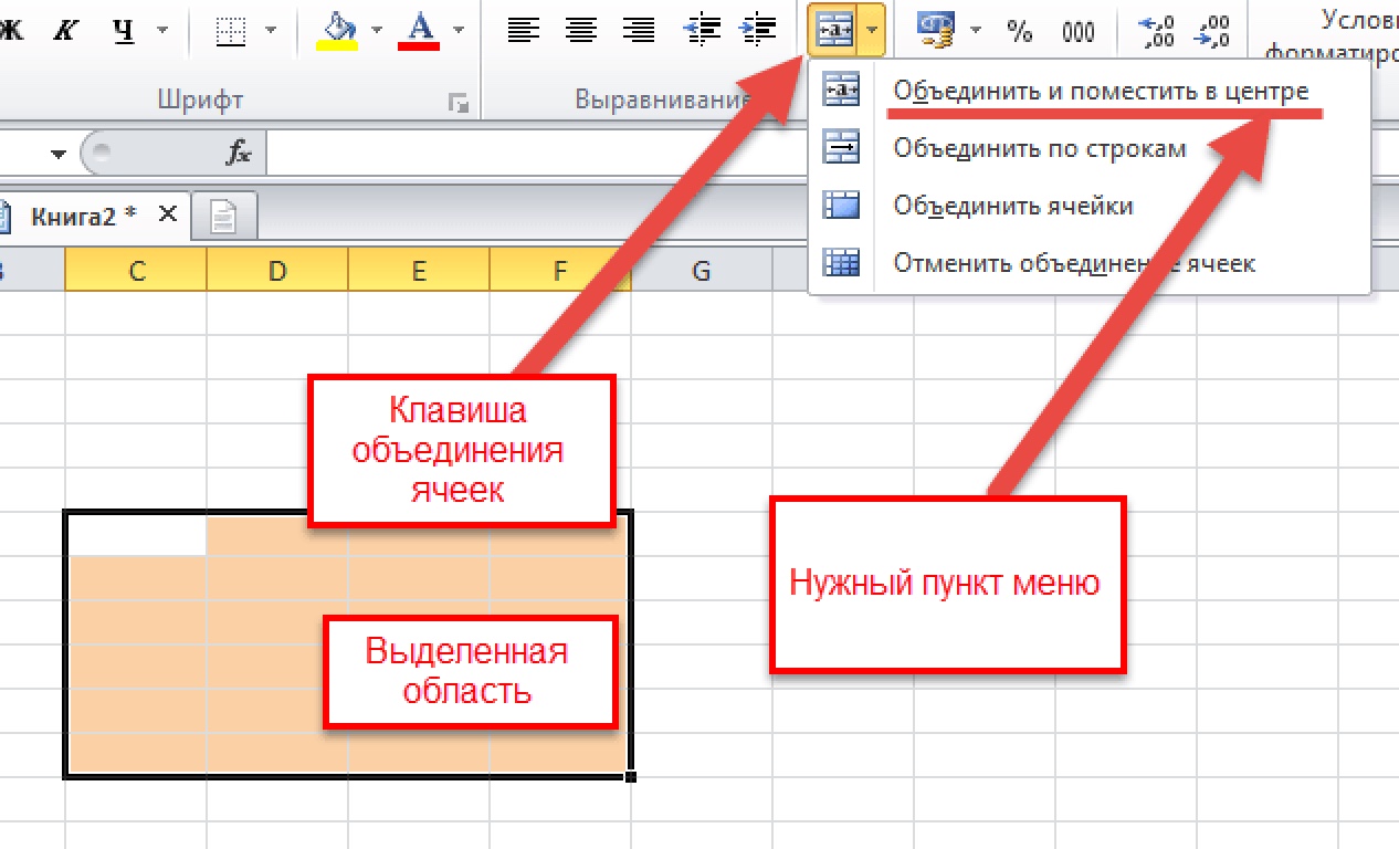
Finding the required button. In the navigation menu, on the “Home” tab, find the button that was marked in the previous screenshot and display the drop-down list. We’ve selected Merge and Center. If this button is inactive, then you need to exit the editing mode. This can be done by pressing the Enter key.
If you need to adjust the position of the text in the resulting large cell, you can do so using the alignment properties found on the Home tab.
Splitting cells
This is a fairly simple procedure that somewhat repeats the previous paragraph:
- Selecting a cell that was previously created by merging several other cells. Separation of others is not possible.
- Once the merged block is selected, the merging key will light up. After clicking on it, all cells will be separated. Each of them will receive their own address. Rows and columns will be recalculated automatically.
Cell Search
It is very easy to overlook important information when you have to work with large amounts of data. To solve this problem, you can use the search. Moreover, you can search not only for words, but also formulas, combined blocks, and anything you like. To do this, you must perform the following steps:
- Make sure the Home tab is open. There is an “Editing” area where you can find the “Find and Select” key.
- After that, a dialog box will open with an input field in which you can enter the value you need. There is also an option to specify additional parameters. For example, if you need to find merged cells, you need to click on “Options” – “Format” – “Alignment”, and check the box next to the search for merged cells.
- The necessary information will be displayed in a special window.
There is also a “Find All” feature to search for all merged cells.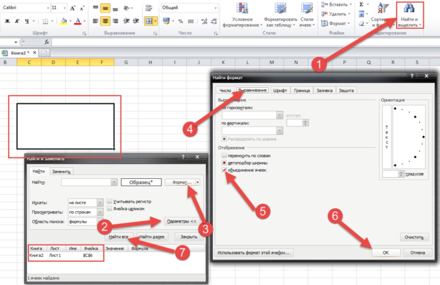
Working with the contents of Excel cells
Here we will look at some functions that allow you to work with input text, functions or numbers, how to perform copy, move and reproduce operations. Let’s look at each of them in order.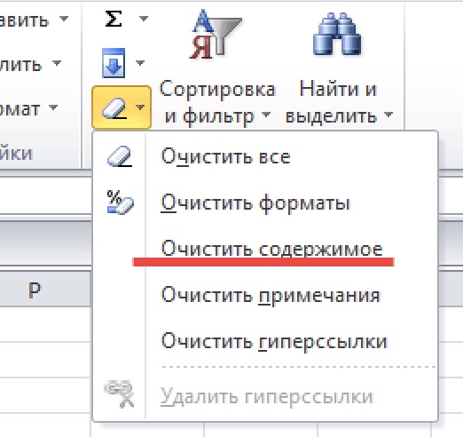
- Input. Everything is simple here. You need to select the desired cell and just start writing.
- Removing information. To do this, you can use both the Delete key and Backspace. You can also use the eraser key in the Editing panel.
- Copy. It is very convenient to carry it out using the Ctrl + C hot keys and paste the copied information to the desired location using the Ctrl + V combination. In this way, rapid data multiplication can be carried out. It can be used not only in Excel, but also in almost any program running Windows. If an incorrect action was performed (for example, an incorrect piece of text was inserted), you can roll back by pressing the Ctrl + Z combination.
- Cutting out. It is carried out using the Ctrl + X combination, after which you need to insert the data in the right place using the same hot keys Ctrl + V. The difference between cutting and copying is that with the latter, the data is stored in the first place, while the cut fragment remains only in the place where it was inserted.
- Formatting. Cells can be changed both outside and inside. Access to all the necessary parameters can be obtained by right-clicking on the required cell. A context menu will appear with all the settings.
Arithmetic operations
Excel is primarily a functional calculator that allows you to perform multi-level calculations. This is especially useful for accounting. This program allows you to perform all conceivable and inconceivable operations with numbers. Therefore, you need to understand how the various functions and characters that can be written to a cell work.
First of all, you need to understand the notation that indicates a particular arithmetic operation:
- + – addition.
- – – subtraction.
- * – multiplication.
- / – division.
- ^ – exponentiation.
- % is a percentage.
Start entering a formula in a cell with an equal sign. For example,
= 7 + 6
After you press the “ENTER” button, the data is automatically calculated and the result is displayed in the cell. If as a result of the calculation it turns out that there are a huge number of digits after the decimal point, then you can reduce the bit depth using a special button on the “Home” tab in the “Number” section.
Using Formulas in Excel
If it is necessary to draw up a final balance, then addition alone is not enough. After all, it consists of a huge amount of data. For this reason, technologies have been developed that make it possible to create a table in just a couple of clicks.
To make it more clear, let’s create such a simple table with data, where you need to calculate several values at once.
To get the final result, simply sum up the values for each item for the first two weeks. This is easy because you can also manually enter a small amount of data. But what, also hands to receive the amount? What needs to be done in order to systematize the available information?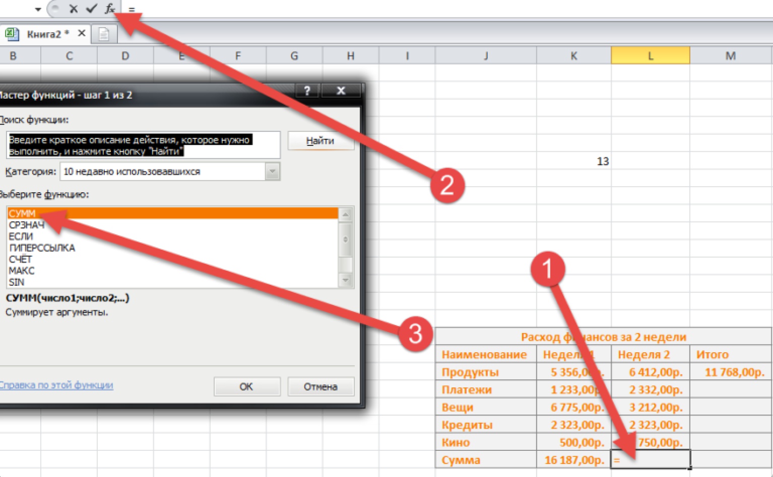
If you use a formula in a cell, you can perform even the most complex calculations, as well as program your document to do whatever you want.
Moreover, the formula can be selected directly from the menu, which is called by pressing the fx button. We have selected the SUM function in the dialog box. To confirm the action, you must press the “Enter” button. Before you actually use the functions, it is recommended to practice a little in the sandbox. That is, create a test document, where you can work out various formulas a bit and see how they work.
Errors when entering a formula in a cell
As a result of entering a formula, various errors may occur:
- ##### – This error is thrown if a value below zero is obtained when entering a date or time. It can also be displayed if there is not enough space in the cell to accommodate all the data.
- #N/A – this error appears if it is impossible to determine the data, as well as if the order of entering the function arguments is violated.
- #LINK! In this case, Excel reports that an invalid column or row address was specified.
- #EMPTY! An error is shown if the arithmetic function was built incorrectly.
- #NUMBER! If the number is excessively small or large.
- #VALUE! Indicates that an unsupported data type is being used. This can happen if one cell that is used for the formula contains text, and the other contains numbers. In this case, the data types do not match each other and Excel starts to swear.
- #DIV/0! – the impossibility of dividing by zero.
- #NAME? – the function name cannot be recognized. For example, there is an error.
Hotkeys
Hotkeys make life easier, especially if you have to repeat the same type of actions often. The most popular hotkeys are as follows:
- CTRL + arrow on the keyboard – select all cells that are in the corresponding row or column.
- CTRL + SHIFT + “+” – insert the time that is on the clock at the moment.
- CTRL + ; – insert current date with automatic filtering function according to Excel rules.
- CTRL + A – select all cells.
Cell appearance settings
Properly chosen cell design allows you to make it more attractive, and the range – easy to read. There are several cell appearance options that you can customize.
Boundaries
The range of spreadsheet features also includes border settings. To do this, click on the cells of interest and open the “Home” tab, where you click on the arrow located to the right of the “Borders” button. After that, a menu will appear in which you can set the necessary border properties.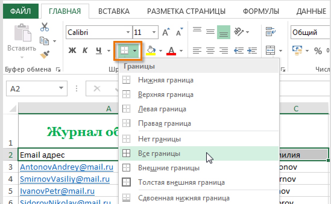
Borders can be drawn. To do this, you need to find the item “Draw Borders”, which is located in this pop-up menu.
Fill color
First you need to select those cells that need to be filled with a certain color. After that, on the “Home” tab, find the arrow located to the right of the “Fill color” item. A pop-up menu will appear with a list of colors. Simply select the desired shade, and the cell will be automatically filled.
Life hack: if you hover over different colors, you can see what the appearance of the cell will be after it is filled with a certain color.
Cell styles
Cell styles are ready-made design options that can be added in a couple of clicks. You can find the menu in the “Home” tab in the “cell styles” section.