


Contents
A matrix is a set of cells located directly next to each other and which together form a rectangle. No special skills are required to perform various actions with the matrix, just the same as those used when working with the classic range are enough.
Each matrix has its own address, which is written in the same way as the range. The first component is the first cell of the range (located in the upper left corner), and the second component is the last cell, which is in the lower right corner.
Array formulas
In the vast majority of tasks, when working with arrays (and matrices are such), formulas of the corresponding type are used. Their basic difference from the usual ones is that the latter output only one value. To apply an array formula, you need to do a few things:
- Select the set of cells where the values will be displayed.
- Direct introduction of the formula.
- Pressing the key sequence Ctrl + Shift + Enter.
After performing these simple steps, an array formula is displayed in the input field. It can be distinguished from the usual curly braces.
To edit, delete array formulas, you need to select the required range and do what you need. To edit a matrix, you need to use the same combination as to create it. In this case, it is not possible to edit a single element of the array.
What can be done with matrices
In general, there are a huge number of actions that can be applied to matrices. Let’s look at each of them in more detail.
Transpose
Many people do not understand the meaning of this term. Imagine that you need to swap rows and columns. This action is called transposition.
Before doing this, it is necessary to select a separate area that has the same number of rows as the number of columns in the original matrix and the same number of columns. For a better understanding of how this works, take a look at this screenshot.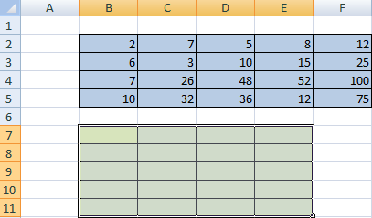
There are several methods for how to transpose.
The first way is the following. First you need to select the matrix, and then copy it. Next, a range of cells is selected where the transposed range should be inserted. Next, the Paste Special window opens.
There are many operations there, but we need to find the “Transpose” radio button. After completing this action, you need to confirm it by pressing the OK button.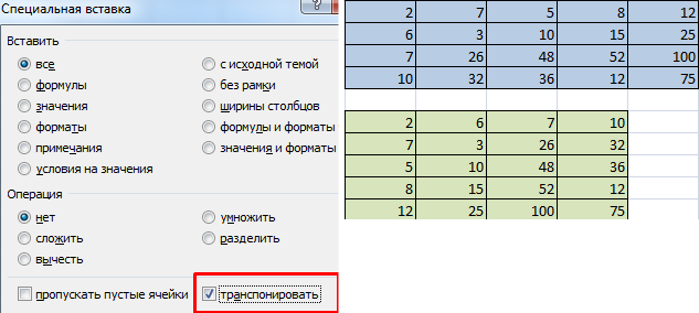
There is another way to transpose a matrix. First you need to select the cell located in the upper left corner of the range allocated for the transposed matrix. Next, a dialog box with functions opens, where there is a function TRANSP. See the example below for more details on how to do this. The range corresponding to the original matrix is used as a function parameter.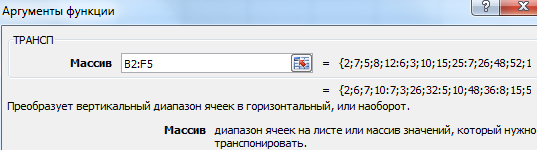
After clicking OK, it will first show that you made a mistake. There is nothing terrible in this. This is because the function we inserted is not defined as an array formula. Therefore, we need to do the following:
- Select a set of cells reserved for the transposed matrix.
- Press the F2 key.
- Press the hot keys Ctrl + Shift + Enter.
The main advantage of the method lies in the ability of the transposed matrix to immediately correct the information contained in it, as soon as the data is entered into the original one. Therefore, it is recommended to use this method.
Addition
This operation is possible only in relation to those ranges, the number of elements of which is the same. Simply put, each of the matrices with which the user is going to work must have the same dimensions. And we provide a screenshot for clarity.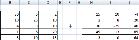
In the matrix that should turn out, you need to select the first cell and enter such a formula.
=First element of the first matrix + First element of the second matrix
Next, we confirm the formula entry with the Enter key and use auto-complete (the square in the lower right corner) to copy all the values uXNUMXbuXNUMXbinto a new matrix.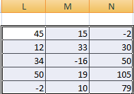
Multiplication
Suppose we have such a table that should be multiplied by 12.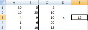
The astute reader can easily understand that the method is very similar to the previous one. That is, each of the cells of matrix 1 must be multiplied by 12 so that in the final matrix each cell contains the value multiplied by this coefficient.
In this case, it is important to specify absolute cell references.
As a result, such a formula will turn out.
=A1*$E$3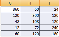
Further, the technique is similar to the previous one. You need to stretch this value to the required number of cells.
Let’s assume that it is necessary to multiply matrices among themselves. But there is only one condition under which this is possible. It is necessary that the number of columns and rows in the two ranges be mirrored the same. That is, how many columns, so many rows.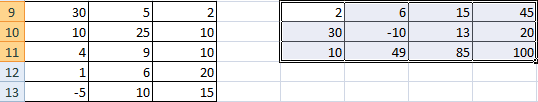
To make it more convenient, we have selected a range with the resulting matrix. You need to move the cursor to the cell in the upper left corner and enter the following formula =MUMNOH(A9:C13;E9:H11). Don’t forget to press Ctrl + Shift + Enter.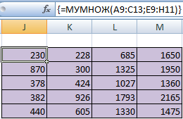
inverse matrix
If our range has a square shape (that is, the number of cells horizontally and vertically is the same), then it will be possible to find the inverse matrix, if necessary. Its value will be similar to the original. For this, the function is used MOBR.
To begin with, you should select the first cell of the matrix, into which the inverse will be inserted. Here is the formula =INV(A1:A4). The argument specifies the range for which we need to create an inverse matrix. It remains only to press Ctrl + Shift + Enter, and you’re done.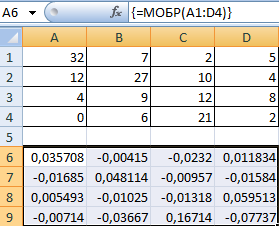
Finding the Determinant of a Matrix
The determinant is a number that is a square matrix. To search for the determinant of a matrix, there is a function − MOPRED.
To begin with, the cursor is placed in any cell. Next, we enter =MOPRED(A1:D4)
A few examples
For clarity, let’s look at some examples of operations that can be performed with matrices in Excel.
Multiplication and division
The 1 method
Suppose we have a matrix A that is three cells high and four cells wide. There is also a number k, which is written in another cell. After performing the operation of multiplying a matrix by a number, a range of values will appear, having similar dimensions, but each part of it is multiplied by k.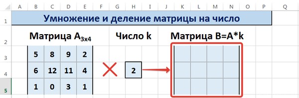
The range B3:E5 is the original matrix that will be multiplied by the number k, which in turn is located in cell H4. The resulting matrix will be in the range K3:N5. The initial matrix will be called A, and the resulting one – B. The latter is formed by multiplying the matrix A by the number k.
Next, enter =B3*$H$4 to cell K3, where B3 is element A11 of matrix A.
Do not forget that cell H4, where the number k is indicated, must be entered into the formula using an absolute reference. Otherwise, the value will change when the array is copied, and the resulting matrix will fail.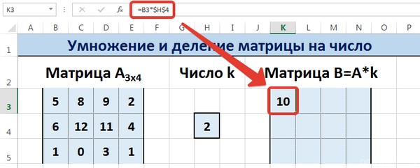
Next, the autofill marker (the same square in the lower right corner) is used to copy the value obtained in cell K3 to all other cells in this range.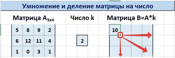
So we managed to multiply the matrix A by a certain number and get the output matrix B.
The division is carried out in a similar way. You just need to enter the division formula. In our case, this =B3/$H$4.
The 2 method
So, the main difference of this method is that the result is an array of data, so you need to apply the array formula to fill the entire set of cells.
It is necessary to select the resulting range, enter the equal sign (=), select the set of cells with the dimensions corresponding to the first matrix, click on the star. Next, select a cell with the number k. Well, to confirm your actions, you must press the above key combination. Hooray, the whole range is filling up.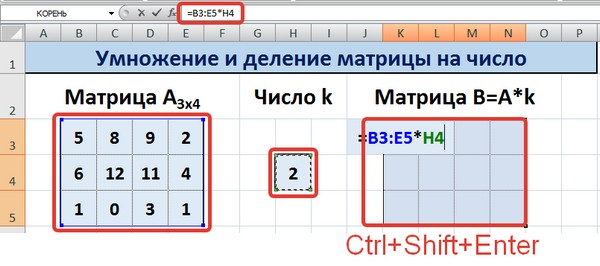
Division is carried out in a similar way, only the sign * must be replaced with /.
Addition and subtraction
Let’s describe some practical examples of using addition and subtraction methods in practice.
The 1 method
Do not forget that it is possible to add only those matrices whose sizes are the same. In the resulting range, all cells are filled with a value that is the sum of similar cells in the original matrices.
Suppose we have two matrices that are 3×4 in size. To calculate the sum, you should insert the following formula into cell N3:
=B3+H3
Here, each element is the first cell of the matrices that we are going to add. It is important that the links are relative, because if you use absolute links, the correct data will not be displayed.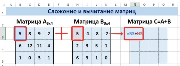
Further, similarly to multiplication, using the autocomplete marker, we spread the formula to all cells of the resulting matrix.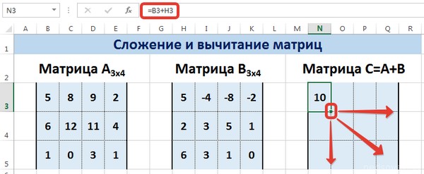
Subtraction is carried out in a similar way, with the only exception that the subtraction (-) sign is used rather than the addition sign.
The 2 method
Similar to the method of adding and subtracting two matrices, this method involves the use of an array formula. Therefore, as its result, a set of values uXNUMXbuXNUMXbwill be issued immediately. Therefore, you cannot edit or delete any elements.
First you need to select the range separated for the resulting matrix, and then click on “=”. Then you need to specify the first parameter of the formula in the form of a range of matrix A, click on the + sign and write the second parameter in the form of a range corresponding to matrix B. We confirm our actions by pressing the combination Ctrl + Shift + Enter. Everything, now the entire resulting matrix is filled with values.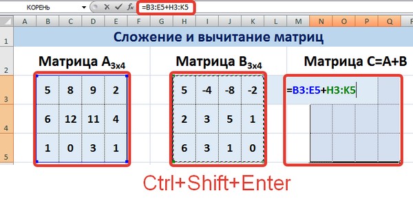
Matrix transposition example
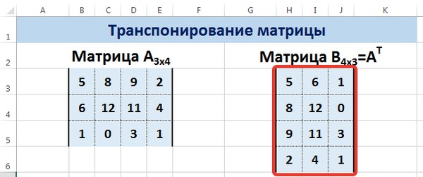
Let’s say we need to create a matrix AT from a matrix A, which we have initially by transposing. The latter has, already by tradition, the dimensions of 3×4. For this we will use the function =TRANSP().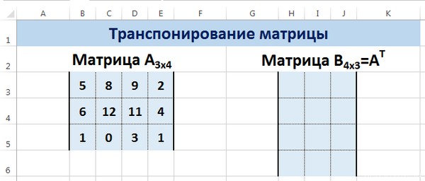
We select the range for the cells of the matrix AT.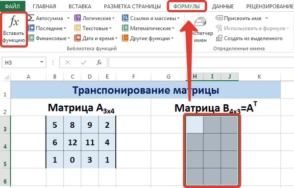
To do this, go to the “Formulas” tab, where select the “Insert function” option, there find the “References and arrays” category and find the function TRANSP. After that, your actions are confirmed with the OK button.
Next, go to the “Function Arguments” window, where the range B3:E5 is entered, which repeats matrix A. Next, you need to press Shift + Ctrl, and then click “OK”.
It’s important. You should not be lazy to press these hot keys, because otherwise only the value of the first cell of the range of the AT matrix will be calculated.
As a result, we get such a transposed table that changes its values after the original one.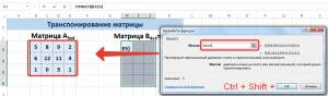
Inverse Matrix Search
Suppose we have a matrix A, which has a size of 3×3 cells. We know that to find the inverse matrix, we need to use the function =MOBR().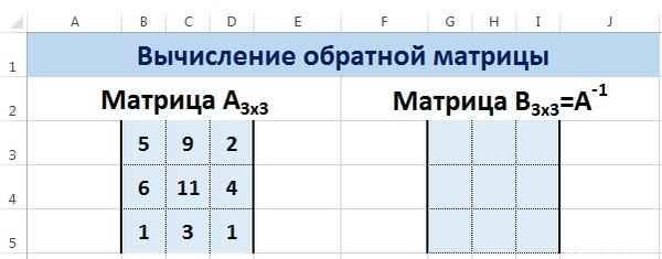
We now describe how to do this in practice. First you need to select the range G3:I5 (the inverse matrix will be located there). You need to find the “Insert Function” item on the “Formulas” tab.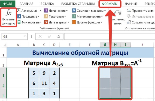
The “Insert function” dialog will open, where you need to select the “Math” category. And there will be a function in the list MOBR. After we select it, we need to press the key OK. Next, the “Function Arguments” dialog box appears, in which we write the range B3: D5, which corresponds to matrix A. Further actions are similar to transposition. You need to press the key combination Shift + Ctrl and click OK.
Conclusions
We have analyzed some examples of how you can work with matrices in Excel, and also described the theory. It turns out that this is not as scary as it might seem at first glance, is it? It just sounds incomprehensible, but in fact, the average user has to deal with matrices every day. They can be used for almost any table where there is a relatively small amount of data. And now you know how you can simplify your life in working with them.