VLOOKUP Function in Excel – Beginner’s Guide: Syntax and Examples

Contents

VLOOKUP function in Excel – general description and syntax
- Syntax of the VLOOKUP function
VLOOKUP Examples
Exact or approximate match in the VLOOKUP function
- Example 1: Finding an Exact Match with VLOOKUP
- Example 2: Using VLOOKUP to Find an Approximate Match
VLOOKUP in Excel – you need to remember this!

Today we are starting a series of articles describing one of the most useful features of Excel − VPR (VLOOKUP). This function, at the same time, is one of the most complex and least understood.

In this tutorial on VPR I will try to lay out the basics as simply as possible in order to make the learning process as clear as possible for inexperienced users. In addition, we will study several examples with Excel formulas that will demonstrate the most common use cases for the function VPR.

VLOOKUP function in Excel – general description and syntax

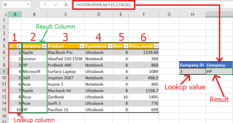
So what is it VPR? Well, first of all, it’s an Excel function. What she does? It looks up the value you specify and returns the corresponding value from the other column. Technically speaking, VPR looks up the value in the first column of the given range and returns the result from another column in the same row.

In the most common application, the function VPR searches the database for a given unique identifier and extracts some information related to it from the database.

First letter in function name VPR (VLOOKUP) means Вvertical (Vvertical). By it you can distinguish VPR from GPR (HLOOKUP), which searches for a value in the top row of a range − Гhorizontal (Hhorizontally).

Function VPR available in Excel 2013, Excel 2010, Excel 2007, Excel 2003, Excel XP, and Excel 2000.

Syntax of the VLOOKUP function

Function VPR (VLOOKUP) has the following syntax:

VLOOKUP(lookup_value,table_array,col_index_num,[range_lookup])

ВПР(искомое_значение;таблица;номер_столбца;[интервальный_просмотр])

As you can see, a function VPR in Microsoft Excel has 4 options (or arguments). The first three are mandatory, the last is optional.

lookup_value (lookup_value) – The value to look for. This can be a value (number, date, text) or a cell reference (containing the lookup value), or a value returned by some other Excel function. For example, this formula will look for the value 40:
=VLOOKUP(40,A2:B15,2)
=ВПР(40;A2:B15;2)

If the lookup value is less than the smallest value in the first column of the range being looked up, the function VPR will report an error #AT (#N/A).

table_array (table) – two or more columns of data. Remember, the function VPR always looks for the value in the first column of the range given in the argument table_array (table). The viewable range can contain various data, such as text, dates, numbers, booleans. The function is case insensitive, meaning upper and lower case characters are considered the same. So our formula will look for the value 40 in cells from A2 to A15, because A is the first column of the range A2:B15 given in the argument table_array (table):
=VLOOKUP(40,A2:B15,2)
=ВПР(40;A2:B15;2)

col_index_num (column_number) is the number of the column in the given range from which the value in the found row will be returned. The leftmost column in the given range is 1, the second column is 2, the third column is 3 and so on. Now you can read the whole formula:
=VLOOKUP(40,A2:B15,2)
=ВПР(40;A2:B15;2)
Formula looking for value 40 in the range A2: A15 and returns the corresponding value from column B (because B is the second column in the range A2:B15).

If the value of the argument col_index_num (column_number) less than 1then VPR will report an error #VALUE! (#VALUE!). And if it is more than the number of columns in the range table_array (table), the function will return an error #REF! (#LINK!).

range_lookup (range_lookup) – determines what to look for:
- exact match, argument must be equal FALSE (FALSE);
- approximate match, argument equals TRUE CODE (TRUE) or not specified at all.
This parameter is optional, but very important. Later in this tutorial on VPR I’ll show you some examples explaining how to write formulas for finding exact and approximate matches.

VLOOKUP Examples

I hope the function VPR become a little clearer to you. Now let’s look at some use cases VPR in formulas with real data.

How to use VLOOKUP to search in another Excel sheet

In practice, formulas with a function VPR are rarely used to search for data on the same worksheet. More often than not, you will be looking up and retrieving corresponding values from another sheet.

In order to use VPR, search in another Microsoft Excel sheet, You must in the argument table_array (table) specify the sheet name with an exclamation mark followed by a range of cells. For example, the following formula shows that the range A2: B15 is on a sheet named Sheet2.

=VLOOKUP(40,Sheet2!A2:B15,2)

=ВПР(40;Sheet2!A2:B15;2)

Of course, the sheet name does not have to be entered manually. Just start typing the formula, and when it comes to the argument table_array (table), switch to the desired sheet and select the desired range of cells with the mouse.

The formula shown in the screenshot below looks for the text “Product 1” in column A (it’s the 1st column of the range A2:B9) on a worksheet Prices.

=VLOOKUP("Product 1",Prices!$A$2:$B$9,2,FALSE)

=ВПР("Product 1";Prices!$A$2:$B$9;2;ЛОЖЬ)

Please remember that when searching for a text value, you must enclose it in quotation marks (“”), as is usually done in Excel formulas.

For argument table_array (table) it is desirable to always use absolute references (with the $ sign). In this case, the search range will remain unchanged when copying the formula to other cells.

Search in another workbook with VLOOKUP

To function VPR worked between two Excel workbooks, you need to specify the workbook name in square brackets before the sheet name.

For example, below is a formula that looks for the value 40 on the sheet Sheet2 in the book Numbers.xlsx:

=VLOOKUP(40,[Numbers.xlsx]Sheet2!A2:B15,2)

=ВПР(40;[Numbers.xlsx]Sheet2!A2:B15;2)

Here is the easiest way to create a formula in Excel with VPRwhich links to another workbook:

Open both books. This is not required, but it is easier to create a formula this way. You don’t want to enter the workbook name manually, do you? In addition, it will protect you from accidental typos.
Start typing a function VPRand when it comes to the argument table_array (table), switch to another workbook and select the required search range in it.

The screenshot below shows the formula with the search set to a range in the workbook PriceList.xlsx on the sheet Prices.

Function VPR will work even when you close the searched workbook and the full path to the workbook file appears in the formula bar, as shown below:

If the name of the workbook or sheet contains spaces, then it must be enclosed in apostrophes:

=VLOOKUP(40,'[Numbers.xlsx]Sheet2'!A2:B15,2)

=ВПР(40;'[Numbers.xlsx]Sheet2'!A2:B15;2)

How to use a named range or table in formulas with VLOOKUP

If you plan to use the same search range in multiple functions VPR, you can create a named range and enter its name into the formula as an argument table_array (table).

To create a named range, simply select the cells and enter an appropriate name in the field First name, to the left of the formula bar.

Now you can write down the following formula for finding the price of a product Product 1:

=VLOOKUP("Product 1",Products,2)

=ВПР("Product 1";Products;2)

Most range names work for the entire Excel workbook, so there is no need to specify the sheet name for the argument table_array (table), even if the formula and the search range are on different worksheets. If they are in different workbooks, then before the name of the range you need to specify the name of the workbook, for example, like this:

=VLOOKUP("Product 1",PriceList.xlsx!Products,2)

=ВПР("Product 1";PriceList.xlsx!Products;2)

So the formula looks much clearer, agree? Also, using named ranges is a good alternative to absolute references because the named range doesn’t change when you copy the formula to other cells. This means that you can be sure that the search range in the formula will always remain correct.

If you convert a range of cells into a full-fledged Excel spreadsheet using the command Table (Table) tab Insertion (Insert), then when you select a range with the mouse, Microsoft Excel will automatically add the column names (or the table name if you select the entire table) to the formula.

The finished formula will look something like this:

=VLOOKUP("Product 1",Table46[[Product]:[Price]],2)

=ВПР("Product 1";Table46[[Product]:[Price]];2)

Or maybe even like this:

=VLOOKUP("Product 1",Table46,2)

=ВПР("Product 1";Table46;2)

When using named ranges, the links will point to the same cells no matter where you copy the function VPR within the workbook.

Using Wildcards in VLOOKUP Formulas

As with many other functions, VPR You can use the following wildcard characters:

Question mark (?) – replaces any single character.
Asterisk (*) – replaces any sequence of characters.

Using Wildcards in Functions VPR can be useful in many cases, for example:

When you do not remember exactly the text you need to find.
When you want to find some word that is part of the content of a cell. Know that VPR searches by the contents of the cell as a whole, as if the option is enabled Match entire cell content (Entire cell) in the standard Excel search.
When a cell contains extra spaces at the beginning or end of the content. In such a situation, you can rack your brains for a long time, trying to figure out why the formula does not work.

Example 1: Looking for text that starts or ends with certain characters

Let’s say you want to search for a specific customer in the database shown below. You don’t remember his last name, but you know that it starts with “ack”. Here is a formula that will do the job just fine:

=VLOOKUP("ack*",$A$2:$C$11,1,FALSE)

=ВПР("ack*";$A$2:$C$11;1;ЛОЖЬ)

Now that you’re sure you’ve found the correct name, you can use the same formula to find the amount paid by this customer. To do this, just change the third argument of the function VPR to the desired column number. In our case, this is column C (3rd in the range):

=VLOOKUP("ack*",$A$2:$C$11,3,FALSE)

=ВПР("ack*";$A$2:$C$11;3;ЛОЖЬ)

Here are some more examples with wildcards:

~ Find a name ending in “man”:

=VLOOKUP("*man",$A$2:$C$11,1,FALSE)

=ВПР("*man";$A$2:$C$11;1;ЛОЖЬ)

~ Find a name that starts with “ad” and ends with “son”:

=VLOOKUP("ad*son",$A$2:$C$11,1,FALSE)

=ВПР("ad*son";$A$2:$C$11;1;ЛОЖЬ)

~ We find the first name in the list, consisting of 5 characters:

=VLOOKUP("?????",$A$2:$C$11,1,FALSE)

=ВПР("?????";$A$2:$C$11;1;ЛОЖЬ)

To function VPR with wildcards worked correctly, as the fourth argument you should always use FALSE (FALSE). If the search range contains more than one value that matches the search terms with wildcards, then the first value found will be returned.

Example 2: Combine wildcards and cell references in VLOOKUP formulas

Now let’s look at a slightly more complex example of how to search using the function VPR by value in a cell. Imagine that column A is a list of license keys, and column B is a list of names that own a license. In addition, you have a part (several characters) of some kind of license key in cell C1, and you want to find the name of the owner.

This can be done using the following formula:

=VLOOKUP("*"&C1&"*",$A$2:$B$12,2,FALSE)

=ВПР("*"&C1&"*";$A$2:$B$12;2;FALSE)

This formula looks up the value from cell C1 in the given range and returns the corresponding value from column B. Note that in the first argument, we use an ampersand (&) character before and after the cell reference to link the text string.

As you can see in the figure below, the function VPR returns “Jeremy Hill” because his license key contains the sequence of characters from cell C1.

Note that the argument table_array (table) in the screenshot above contains the name of the table (Table7) instead of specifying a range of cells. This is what we did in the previous example.

Exact or approximate match in the VLOOKUP function

And finally, let’s take a closer look at the last argument that is specified for the function VPR – range_lookup (interval_view). As mentioned at the beginning of the lesson, this argument is very important. You can get completely different results in the same formula with its value TRUE CODE (TRUE) or FALSE (FALSE).

First, let’s find out what Microsoft Excel means by exact and approximate matches.

If the argument range_lookup (range_lookup) is equal to FALSE (FALSE), the formula looks for an exact match, i.e. exactly the same value as given in the argument lookup_value (lookup_value). If in the first column of the range table_array (table) encounters two or more values that match the argument lookup_value (search_value), then the first one will be selected. If no matches are found, the function will report an error #AT (#N/A). For example, the following formula will report an error #AT (#N/A) if there is no value in the range A2:A15 4:
=VLOOKUP(4,A2:B15,2,FALSE)
=ВПР(4;A2:B15;2;ЛОЖЬ)
If the argument range_lookup (range_lookup) is equal to TRUE CODE (TRUE), the formula looks for an approximate match. More precisely, first the function VPR looks for an exact match, and if none is found, selects an approximate one. An approximate match is the largest value that does not exceed the value specified in the argument. lookup_value (lookup_value).

If the argument range_lookup (range_lookup) is equal to TRUE CODE (TRUE) or not specified, then the values in the first column of the range should be sorted in ascending order, that is, from smallest to largest. Otherwise, the function VPR may return an erroneous result.

To better understand the importance of choice TRUE CODE (TRUTH) or FALSE (FALSE), let’s look at some more formulas with the function VPR and look at the results.

Example 1: Finding an Exact Match with VLOOKUP

As you remember, to search for an exact match, the fourth argument of the function VPR should matter FALSE (FALSE).

Let’s go back to the table from the very first example and find out which animal can move at a speed 50 miles per hour. I believe that this formula will not cause you any difficulties:

=VLOOKUP(50,$A$2:$B$15,2,FALSE)

=ВПР(50;$A$2:$B$15;2;ЛОЖЬ)

Note that our search range (column A) contains two values 50 – in cells A5 и A6. Formula returns value from cell B5. Why? Because when looking for an exact match, the function VPR uses the first value found that matches the one being searched for.

Example 2: Using VLOOKUP to Find an Approximate Match

When you use the function VPR to search for an approximate match, i.e. when the argument range_lookup (range_lookup) is equal to TRUE CODE (TRUE) or omitted, the first thing you need to do is sort the range by the first column in ascending order.

This is very important because the function VPR returns the next largest value after the given one, and then the search stops. If you neglect the correct sorting, you will end up with very strange results or an error message. #AT (#N/A).

Now you can use one of the following formulas:

=VLOOKUP(69,$A$2:$B$15,2,TRUE) or =VLOOKUP(69,$A$2:$B$15,2)

=ВПР(69;$A$2:$B$15;2;ИСТИНА) or =ВПР(69;$A$2:$B$15;2)

As you can see, I want to find out which of the animals has the closest speed to 69 miles per hour. And here is the result the function returned to me VPR:

As you can see, the formula returned a result Antelope (Antelope), whose speed 61 miles per hour, although the list also includes Cheetah (Cheetah) who runs at speed 70 miles per hour, and 70 is closer to 69 than 61, isn’t it? Why is this happening? Because the function VPR when searching for an approximate match, returns the largest value that is not greater than the one being searched for.

I hope these examples shed some light on working with the function VPR in Excel, and you no longer look at her as an outsider. Now it does not hurt to briefly repeat the key points of the material we have studied in order to better fix it in memory.

VLOOKUP in Excel – you need to remember this!

Function VPR Excel can’t look left. It always looks for the value in the leftmost column of the range given by the argument table_array (table).
In function VPR all values are case-insensitive, i.e. small and large letters are equivalent.
If the value you are looking for is less than the minimum value in the first column of the range being looked up, the function VPR will report an error #AT (#N/A).
If 3rd argument col_index_num (column_number) less than 1function VPR will report an error #VALUE! (#VALUE!). If it is greater than the number of columns in the range table_array (table), the function will report an error #REF! (#LINK!).
Use absolute cell references in argument table_array (table) so that the correct search range is preserved when copying the formula. Try using named ranges or tables in Excel as an alternative.
When doing an approximate match search, remember that the first column in the range you are looking for must be sorted in ascending order.
Finally, remember the importance of the fourth argument. Use values TRUE CODE (TRUTH) or FALSE (FALSE) deliberately and you will get rid of many headaches.

In the following articles of our function tutorial VPR in Excel, we will learn more advanced examples, such as performing various calculations using VPR, extracting values from multiple columns, and more. Thank you for reading this tutorial and I hope to see you again next week!