Using the VIEW function in Excel

The Excel program allows you not only to enter data into a table, but also to process them in various ways. As part of this publication, we will consider why the function is needed VIEW and how to use it.

Practical benefits

VIEW is used to find and display a value from the table being searched for by processing/matching a user-specified parameter. For example, we enter the name of a product in a separate cell, and its price, quantity, etc. automatically appear in the next cell. (depending on what we need).

Function VIEW somewhat similar to , but it doesn’t care if the values ​​it looks up are exclusively in the leftmost column.

Using the VIEW function

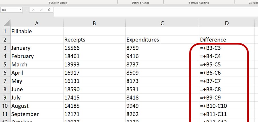
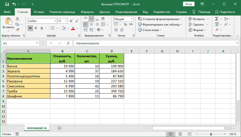
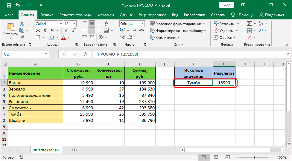
Let’s say we have a table with the names of goods, their price, quantity and amount.

Note: the data to be searched must be arranged strictly in ascending order, otherwise the function VIEW will not work correctly, that is:

• Numbers: … -2, -1, 0, 1, 2…
• Letters: from A to Z, from A to Z, etc.
• Boolean expressions: FALSE, TRUE.

You can use .

There are two ways to apply the function VIEW: vector form and array form. Let’s take a closer look at each of them.

Method 1: vector shape

Excel users most often use this method. Here is what it is:

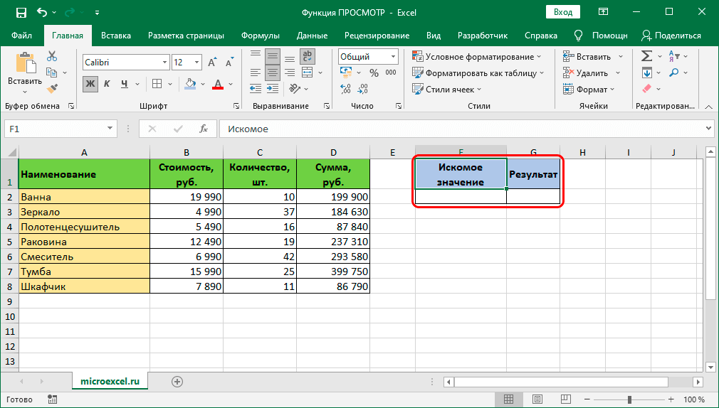
1. Next to the original table, create another one, the header of which contains columns with names “Desired value” и “Result”. In fact, this is not a prerequisite, however, it is easier to work with the function this way. Heading names may also be different.
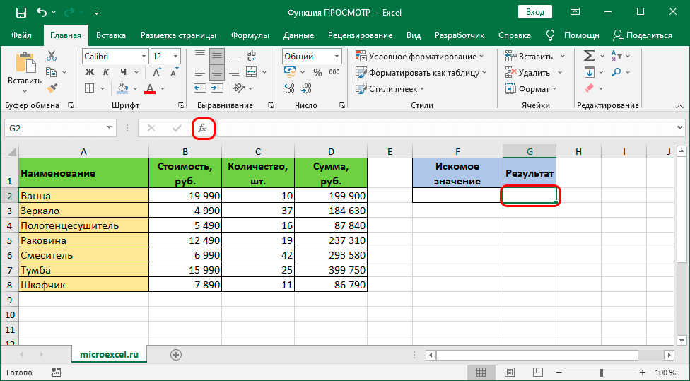
2. We stand in the cell in which we plan to display the result, and then click on the icon “Insert function” to the left of the formula bar.
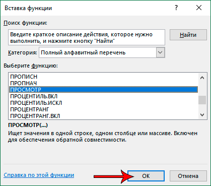
3. A window will appear in front of us Function Wizards. Here we select a category “Full alphabetical list”, scroll down the list, find the operator “VIEW”, mark it and click OK.
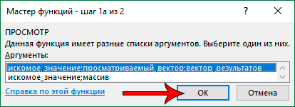
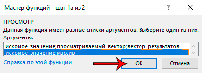
4. A small window will appear on the screen in which we need to select one of the two lists of arguments. In this case, we stop at the first option, because. parsing a vector shape.
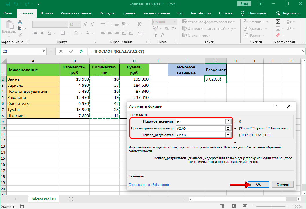
5. Now we need to fill in the arguments of the function, and then click the button OK:
   • “Lookup_value” – here we indicate the coordinates of the cell (we write it manually or simply click on the desired element in the table itself), into which we will enter the parameter by which the search will be performed. In our case, this is “F2”.
   • “Viewed_Vector” – specify the range of cells among which the search for the desired value will be performed (we have this “A2:A8”). Here we can also enter the coordinates manually, or select the required area of ​​cells in the table with the left mouse button held down.
   • “result_vector” – here we indicate the range from which to select the result corresponding to the desired value (will be in the same line). In our case, let’s “Quantity, pcs.”, i.e. range “C2:C8”.
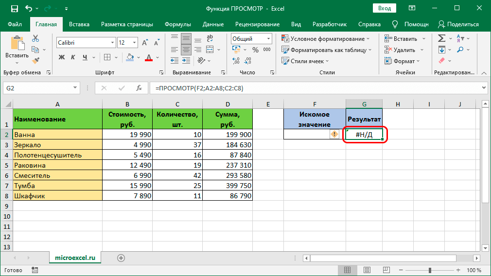
6. In the cell with the formula, we see the result “#N/A”, which may be perceived as an error, but it is not entirely true.
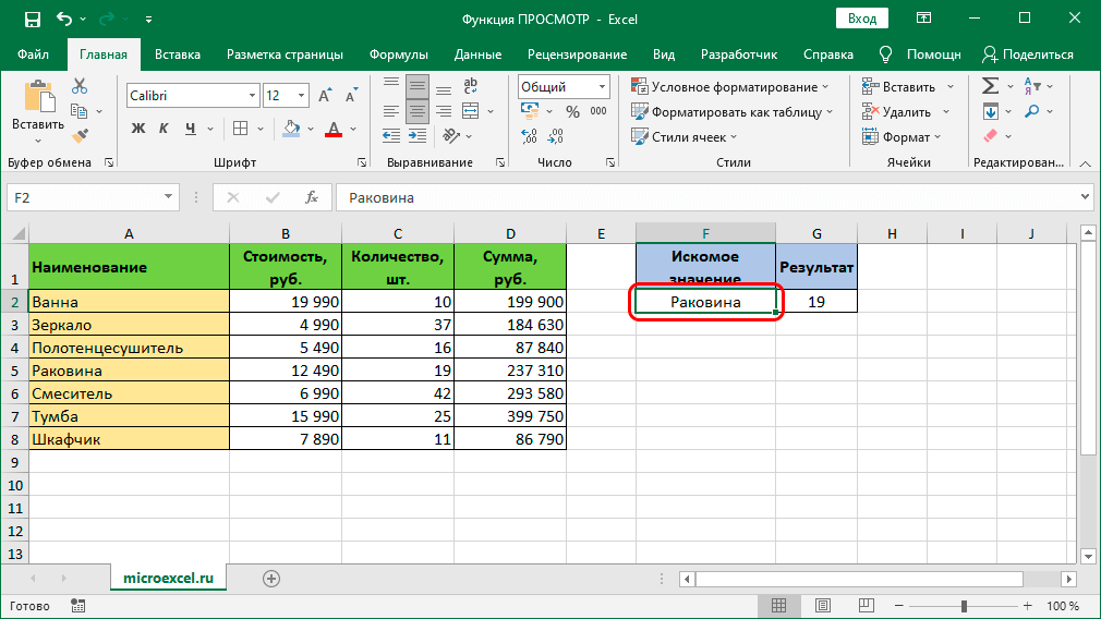
7. For the function to work, we need to enter into the cell “F2” some name (for example, “Sink”) contained in the source table, case is not important. After we click Enter, the function will automatically pull up the desired result (we will have it 19 pc).Note: experienced users can do without Function Wizards and immediately enter the function formula in the appropriate line with links to the required cells and ranges.

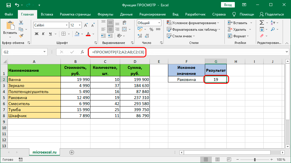
Method 2: Array Form

In this case, we will work immediately with the whole array, which simultaneously includes both ranges (viewed and results). But there is a significant limitation here: the viewed range must be the outermost column of the given array, and the selection of values ​​will be performed from the rightmost column. So, let’s get to work:

1. Insert a function into the cell to display the result VIEW – as in the first method, but now we select the list of arguments for the array.
2. Specify the function arguments and click the button OK:
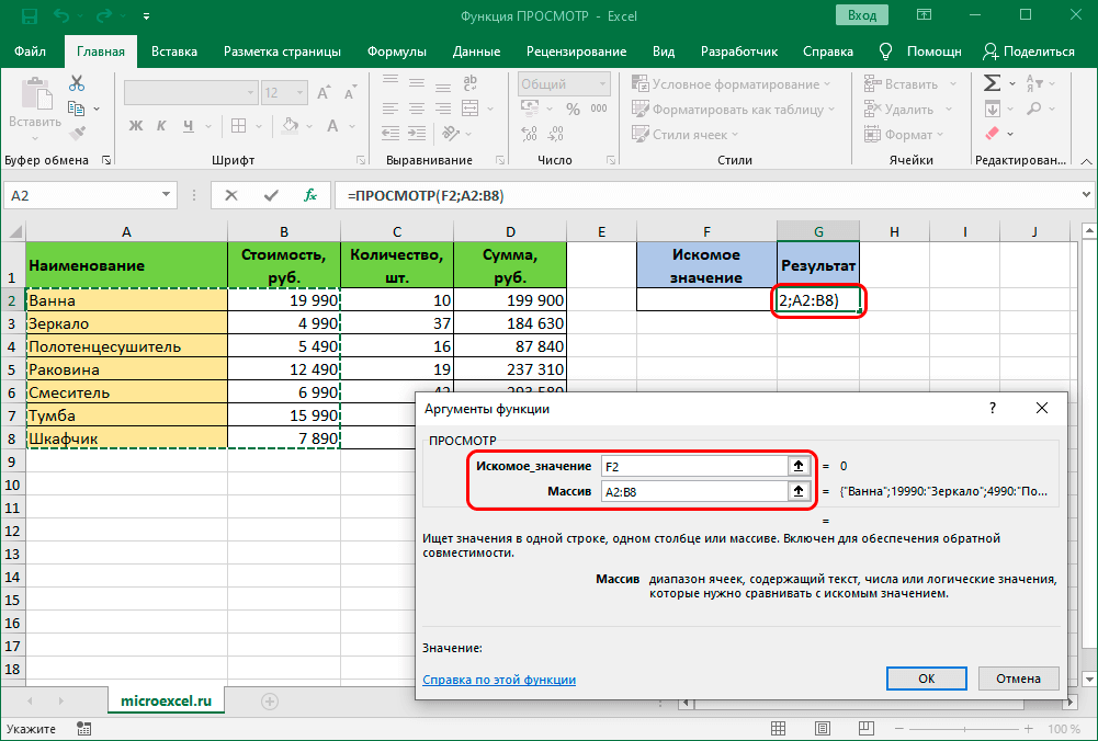
   • “Lookup_value” – filled in the same way as for the vector form.
   • “Array” – set the coordinates of the entire array (or select it in the table itself), including the range being viewed and the results area.
3. To use the function, as in the first method, enter the name of the product and click Enter, after which the result will automatically appear in the cell with the formula.

Note: array form for function VIEW rarely used, tk. is obsolete and remains in modern versions of Excel to maintain compatibility with workbooks created in earlier versions of the program. Instead, it is desirable to use modern functions: VPR и GPR.

Conclusion

Thus, in Excel there are two ways to use the LOOKUP function, depending on the selected list of arguments (vector form or range form). By learning how to use this tool, in some cases, you can significantly reduce the processing time of information, paying attention to more important tasks.