


Contents
Formulation of the problem
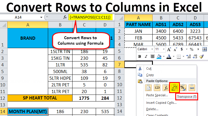
We want, to put it simply, to turn the table on its side, i.e. what was located in the row – let it go through the column and vice versa:
Method 1: Paste Special
Select and copy the source table (right-click – Copy). Then we right-click on the empty cell where we want to place the rotated table and select the command from the context menu Paste special (Paste Special). In the dialog box that opens, check the box Transpose (Transpose) and click OK.
Cons: cells with formulas are not always copied correctly, there is no connection between tables (changing data in the first table will not affect the second).
Pros: The transposed table retains the original cell formatting.
Method 2. Function TRANSP
Select the required number of empty cells (i.e. if, for example, the original table had 3 rows and 5 columns, then you must select a range of 5 rows and 3 columns) and enter the function in the first cell TRANSP (TRANSPOSE) from category References and arrays (Lookup and Reference):
After entering the function, you must press not Enter, but Ctrl + Shift + Enterto enter it at once in all selected cells as array formula. If you have not encountered array formulas before, then I advise read here is a very exotic but very powerful tool in Excel.
Pros: the relationship between the tables is maintained, i.e. changes in the first table are immediately reflected in the second.
Cons: formatting is not preserved, empty cells from the first table are displayed as zeros in the second table, individual cells in the second table cannot be edited, since the array formula can only be changed in its entirety.
Method 3. We form the address ourselves
This method is somewhat similar to the previous one, but allows you to freely edit the values in the second table and make any changes to it if necessary. To create links to rows and columns, we need four functions from the category References and arrays:
- Function ADDRESS(line_number; column_number) – gives the address of the cell by the number of the row and column on the sheet, i.e. ADDRESS(2;3) will give, for example, a link to cell C2.
- Function INDIRECT(text_link) – converts a text string, for example, “F3” into a real reference to cell F3.
- functions ROW(cell) и COLUMN(cell) – give the row and column number for the given cell, for example =ROW(F1) will return 1, and =COLUMN(A3) will return 3.
Now we connect these functions to get the link we need, i.e. Enter the following formula into any empty cell:
=INDIRECT(ADDRESS(COLUMN(A1),ROW(A1)))
in the English version of Excel it would be =INDIRECT(ADDRESS(COLUMN(A1),ROW(A1)))
And then we copy (stretch) the formula to neighboring cells as usual with a black cross. The result should be something like this:
Those. when copying a formula down a column, it produces a link that goes right down the row and vice versa. What was required.
Pros: relationships between tables are preserved, you can easily make changes to the second table.
Cons: Formatting is not retained but can be easily reproduced special insert (insert only Framework with a flag Transpose