


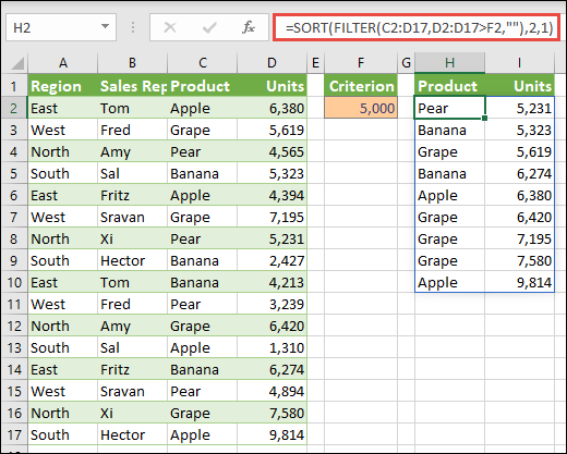
If you need to sort the list, then there are a lot of ways at your service, the easiest of which is the sort buttons on the tab or in the menu Data (Data — Sort). However, there are situations when the sorting of the list needs to be done automatically, i.e. formulas. This may be required, for example, when generating data for a drop-down list, when calculating data for charts, etc. How to sort a list with a formula on the fly?
Method 1. Numeric data
If the list contains only numeric information, then sorting it can be easily done using the functions LEAST (SMALL) и LINE (ROW):
Function LEAST (SMALL) pulls out from the array (column A) the n-th smallest element in a row. Those. SMALL(A:A;1) is the smallest number in the column, SMALL(A:A;2) is the second smallest, and so on.
Function LINE (ROW) returns the row number for the specified cell, i.e. ROW(A1)=1, ROW(A2)=2 etc. In this case, it is used simply as a generator of a sequence of numbers n=1,2,3… for our sorted list. With the same success, it was possible to make an additional column, fill it manually with the numerical sequence 1,2,3 … and refer to it instead of the ROW function.
Method 2. Text list and regular formulas
If the list contains not numbers, but text, then the SMALL function will no longer work, so you have to go a different, slightly longer, path.
First, let’s add a service column with a formula where the serial number of each name in the future sorted list will be calculated using the function COUNTIF (COUNTIF):
In the English version it will be:
=COUNTIF(A:A,»<"&A1)+COUNTIF($A$1:A1,"="&A1)
The first term is a function for counting the number of cells that are less than the current one. The second is a safety net in case any name occurs more than once. Then they will not have the same, but successively increasing numbers.
Now the received numbers must be arranged sequentially in ascending order. For this you can use the function LEAST (SMALL) from the first way:
Well, finally, it remains just to pull out the names from the list by their numbers. To do this, you can use the following formula:
Function MORE EXPOSED (MATCH) searches in column B for the desired serial number (1, 2, 3, etc.) and, in fact, returns the number of the line where this number is located. Function INDEX (INDEX) pulls out from column A the name at this line number.
Method 3: Array Formula
This method is, in fact, the same placement algorithm as in Method-2, but implemented by an array formula. To simplify the formula, the range of cells C1:C10 was given the name List (select cells, press Ctrl + F3 and button Create):
In cell E1, copy our formula:
=INDEX(List; MATCH(SMALL(COUNTIF(List; “<"&List); ROW(1:1)); COUNTIF(List; "<"&List); 0))
Or in the English version:
=INDEX(List, MATCH(SMALL(COUNTIF(List, «<"&List), ROW(1:1)), COUNTIF(List, "<"&List), 0))
and push Ctrl + Shift + Enterto enter it as an array formula. Then the resulting formula can be copied down the entire length of the list.
If you want the formula to take into account not a fixed range, but be able to adjust when adding new elements to the list, then you will need to slightly change the strategy.
First, the List range will need to be set dynamically. To do this, when creating, you need to specify not a fixed range C3:C10, but a special formula that will refer to all available values, regardless of their number. Click Alt + F3 or open the tab Formulas – Name Manager (Formulas — Name Manager), create a new name and in the field Link (Reference) enter the following formula (I assume that the range of data to be sorted starts from cell C1):
=СМЕЩ(C1;0;0;СЧЁТЗ(C1:C1000);1)
=OFFSET(C1,0,0,SCHÖTZ(C1:C1000),1)
Secondly, the above array formula will need to be stretched down with a margin – with the expectation of additional data entered in the future. In this case, the array formula will start to give an error #NUMBER on cells that are not yet filled. To intercept it, you can use the function IFERROR, which needs to be added “around” our array formula:
=IFERROR(INDEX(List; MATCH(SMALL(COUNTIF(List; “<"&List); ROW(1:1)); COUNTIF(List; "<"&List); 0));»»)
=IFERROR(NDEX(List, MATCH(SMALL(COUNTIF(List, «<"&List), ROW(1:1)), COUNTIF(List, "<"&List), 0));"")
It catches the #NUMBER error and outputs a void (empty quotes) instead.
:
- Sort range by color
- What are array formulas and why are they needed
- SORT sorting and dynamic arrays in the new Office 365