Sensitivity Analysis in Excel (Sample Datasheet)

Processes in the field of finance are always interconnected – one factor depends on another and changes with it. Track these changes and understand what to expect in the future, perhaps using Excel functions and spreadsheet methods.

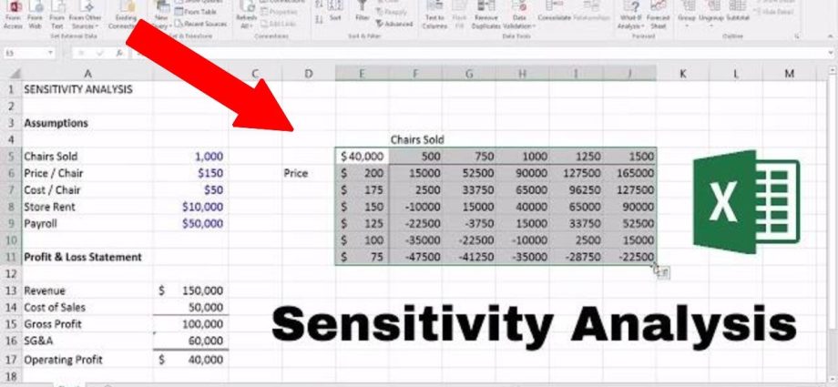
Getting multiple results with a data table

Datasheet capabilities are elements of what-if analysis—often done through Microsoft Excel. This is the second name for sensitivity analysis.

Overview

A data table is a type of range of cells that can be used to solve problems by changing the values ​​in some cells. It is created when it is necessary to keep track of changes in the components of the formula and receive updates to the results, according to these changes. Let’s find out how to use data tables in research, and what types they are.

Basics about data tables

There are two types of data tables, they differ in the number of components. You need to compile a table with a focus on the number of values ​​uXNUMXbuXNUMXbthat you need to check with it.

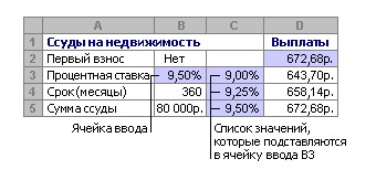
Statisticians use a single variable table when there is only one variable in one or more expressions that can change their result. For example, it is often used in conjunction with the PMT function. The formula is designed to calculate the amount of the regular payment and takes into account the interest rate specified in the agreement. In such calculations, the variables are written in one column, and the results of the calculations in another. An example of a data plate with 1 variable:

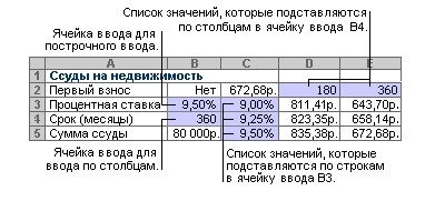
Next, consider the plates with 2 variables. They are used in cases where two factors influence the change in any indicator. The two variables may end up in another table associated with the loan, which can be used to determine the optimal repayment period and the amount of the monthly payment. In this calculation, you also need to use the PMT function. An example of a table with 2 variables:

Creating a data table with one variable

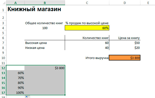
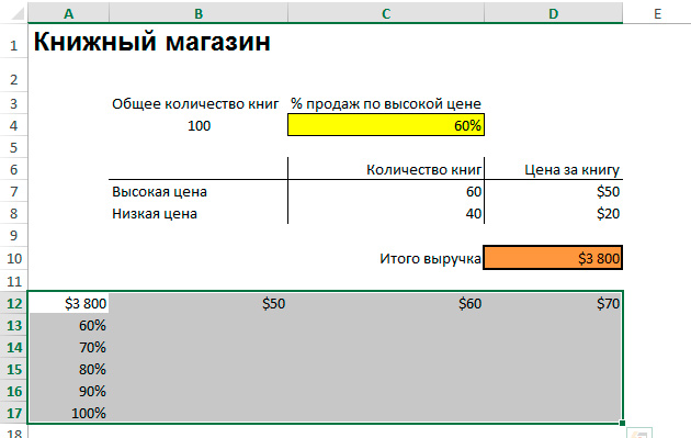
Consider the analysis method using the example of a small bookstore with only 100 books in stock. Some of them can be sold more expensive ($50), the rest will cost buyers less ($20). The total income from the sale of all goods is calculated – the owner decided that he would sell 60% of the books at a high price. You need to find out how revenue will increase if you increase the price of a larger volume of goods – 70%, and so on.

Pay attention! The total revenue must be calculated using a formula, otherwise it will not be possible to compile a data table.

1. Select a free cell away from the edge of the sheet and write the formula in it: =Cell of total revenue. For example, if income is written in cell C14 (random designation is indicated), you need to write this: =S14.
2. We write the percentage of the volume of goods in the column to the left of this cell – not below it, this is very important.
3. We select the range of cells where the percentage column and the link to the total income are located.

4. We find on the “Data” tab the item “What if analysis” and click on it – in the menu that opens, select the option “Data table”.

5. A small window will open where you need to specify a cell with the percentage of books initially sold at a high price in the “Substitute values ​​by rows in …” column. This step is done in order to recalculate the total revenue taking into account the increasing percentage.

After clicking the “OK” button in the window where the data was entered for compiling the table, the results of the calculations will appear in the lines.

Adding a Formula to a Single Variable Data Table

From a table that helped calculate an action with only one variable, you can make a sophisticated analysis tool by adding an additional formula. It must be entered next to an already existing formula – for example, if the table is row-oriented, we enter the expression in the cell to the right of the existing one. When the column orientation is set, we write the new formula under the old one. Next, follow the algorithm:

1. Select the range of cells again, but now it should include the new formula.
2. Open the “what if” analysis menu and select “Datasheet”.
3. We add a new formula to the corresponding field in rows or columns, depending on the orientation of the plate.

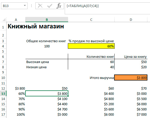
Create a data table with two variables

The start of such a table is slightly different – you need to put a link to the total revenue above the percentage values. Next, we perform these steps:

1. Write price options in one line with a link to income – one cell for each price.
2. Select a range of cells.

3. Open the data table window, as when compiling a table with one variable – through the “Data” tab on the toolbar.
4. Substitute in the column “Substitute values ​​by columns in …” a cell with an initial high price.
5. Add a cell with the initial percentage of sales of expensive books to the “Substitute values ​​by rows in …” column and click “OK”.

As a result, the entire table is filled with amounts of possible income with different conditions for the sale of goods.

Speed ​​up calculations for worksheets containing data tables

If you need quick calculations in a data table that don’t trigger a recalculation of the entire workbook, there are a few things you can do to speed up the process.

1. Open the options window, select the item “Formulas” in the menu on the right.
2. Select the item “Automatic, except for data tables” in the “Computations in the workbook” section.

3. Let’s recalculate the results in the table manually. To do this, select the formulas and press the F key.

Other Tools for Performing Sensitivity Analysis

There are other tools in the program to help you perform sensitivity analysis. They automate some actions that would otherwise have to be done manually.

1. The “Parameter selection” function is suitable if the desired result is known, and you need to know the input value of the variable to obtain such a result.
2. “Search for a solution” is an add-on for solving problems. It is necessary to set limits and point to them, after which the system will find the answer. The solution is determined by changing the values.
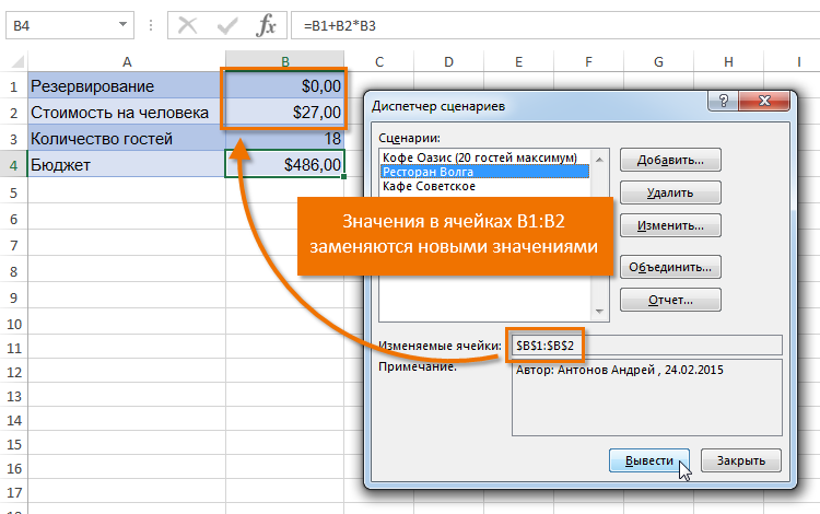
3. Sensitivity analysis can be done using the Scenario Manager. This tool is found in the what-if analysis menu under the Data tab. It substitutes values ​​in several cells – the number can reach 32. The dispatcher compares these values ​​so that the user does not have to change them manually. An example of using the script manager:

Sensitivity analysis of an investment project in Excel

What-if analysis is especially useful in situations where forecasting is required, such as investment. Analysts use this method to find out how the value of a company’s stock will change as a result of changes in some factors.

Investment Sensitivity Analysis Method

When analyzing “what if” use enumeration – manual or automatic. The range of values ​​is known, and they are substituted into the formula one by one. The result is a set of values. Choose the appropriate number from them. Let’s consider four indicators for which sensitivity analysis is carried out in the field of finance:

1. Net Present Value – Calculated by subtracting the amount of the investment from the amount of income.
2. Internal rate of return / profit – indicates how much profit is required to be received from an investment in a year.
3. The payback ratio is the ratio of all profits to the initial investment.
4. Discounted profit index – indicates the effectiveness of the investment.

Formula

Embedding sensitivity can be calculated using this formula: Change in output parameter in % / Change in input parameter in %.

The output and input parameters can be the values ​​described earlier.

1. You need to know the result under standard conditions.
2. We replace one of the variables and monitor the changes in the result.
3. We calculate the percentage change of both parameters relative to the established conditions.
4. We insert the obtained percentages into the formula and determine the sensitivity.

An example of sensitivity analysis of an investment project in Excel

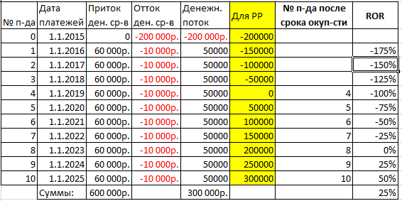
For a better understanding of the analysis methodology, an example is needed. Let’s analyze the project with the following known data:

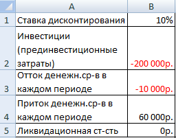
1. Fill in the table to analyze the project on it.

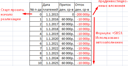
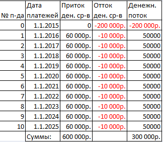
2. We calculate the cash flow using the OFFSET function. At the initial stage, the flow is equal to the investments. Next, we apply the formula: =IF(OFFSET(Number,1;)=2;SUM(Inflow 1:Outflow 1); SUM(Inflow 1:Outflow 1)+$B$5)
   Cell designations in the formula may be different, depending on the layout of the table. At the end, the value from the initial data is added – the salvage value.

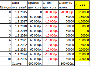
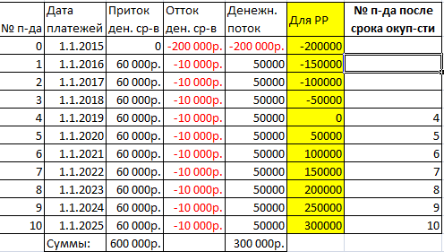
3. We determine the period for which the project will pay off. For the initial period, we use this formula: =SUMMESLY(G7: G17;»<0″). The cell range is the cash flow column. For further periods, we apply this formula: =Initial period+IF(First e.stream>0; First e.stream;0). The project is at the break-even point in 4 years.

4. We create a column for the numbers of those periods when the project pays off.

5. We calculate the return on investment. It is necessary to make an expression where the profit in a particular period of time is divided by the initial investment.

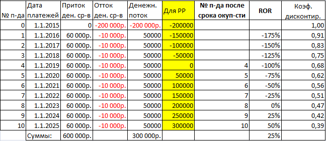
6. We determine the discount factor using this formula: =1/(1+Disc.%) ^Number.

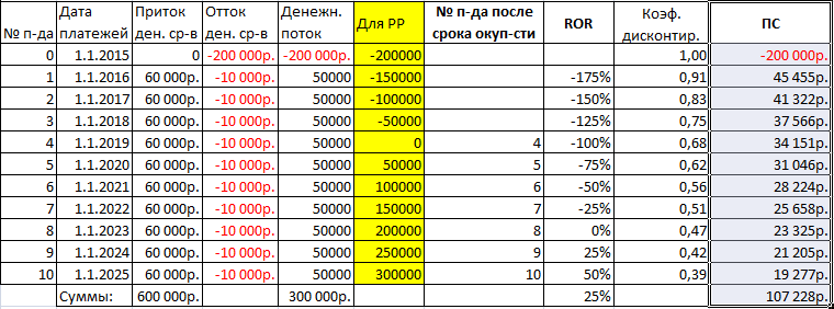
7. We calculate the present value using multiplication – the cash flow is multiplied by the discount factor.

8. Let’s calculate PI (profitability index). The present value over time is divided by the investment at the start of the project.

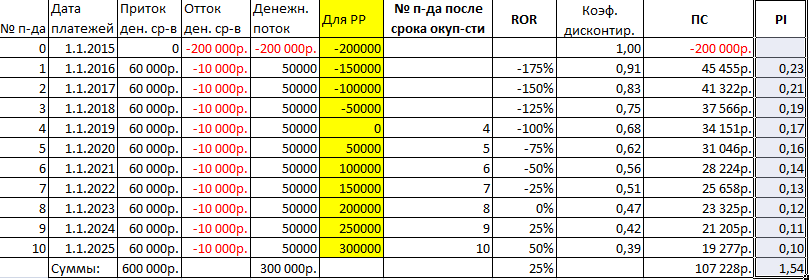
9. Let’s define the internal rate of return using the IRR function: =IRR(Range of cash flow).

Investment Sensitivity Analysis Using Datasheet

For the analysis of projects in the field of investment, other methods are better suited than a data table. Many users experience confusion when compiling a formula. To find out the dependence of one factor on changes in others, you need to select the correct cells for entering calculations and for reading data.

Factor and dispersion analysis in Excel with calculation automation

Another typology of sensitivity analysis is factor analysis and analysis of variance. The first type defines the relationship between numbers, the second reveals the dependence of one variable on others.

ANOVA in Excel

The purpose of such an analysis is to divide the variability of the value into three components:

1. Variability as a result of the influence of other values.
2. Changes due to the relationship of the values ​​that affect it.
3. Random changes.

Let’s perform analysis of variance through the Excel add-in “Data Analysis”. If it is not enabled, it can be enabled in the settings.

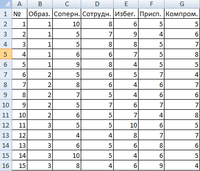
The initial table must follow two rules: there is one column for each value, and the data in it is arranged in ascending or descending order. It is necessary to check the influence of the level of education on behavior in conflict.

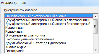
1. Find the Data Analysis tool in the Data tab and open its window. In the list, you need to select one-way analysis of variance.

2. Fill in the lines of the dialog box. The input interval is all cells, excluding headers and numbers. Group by columns. We display the results on a new sheet.

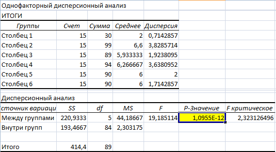
Since the value in the yellow cell is greater than one, the assumption can be considered incorrect – there is no relationship between education and behavior in conflict.

Factor analysis in Excel: an example

Let’s analyze the relationship of data in the field of sales – it is necessary to identify popular and unpopular products. Initial information:

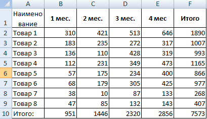
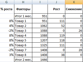
1. We need to find out for which goods demand increased the most during the second month. We are compiling a new table to determine the growth and decline in demand. Growth is calculated using this formula: =IF((Demand 2-Demand 1)>0; Demand 2- Demand 1;0). Decrease formula: =IF(Growth=0; Demand 1- Demand 2;0).

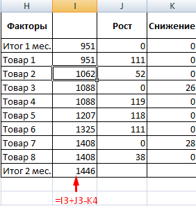
2. Calculate the growth in demand for goods as a percentage: =IF(Growth/Outcome 2 =0; Decrease/Outcome 2; Growth/Outcome 2).

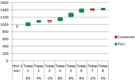
3. Let’s make a chart for clarity – select a range of cells and create a histogram through the “Insert” tab. In the settings, you need to remove the fill, this can be done through the Format Data Series tool.

Two-way analysis of variance in Excel

Analysis of variance is carried out with several variables. Consider this with an example: you need to find out how quickly the reaction to a sound of different volume manifests itself in men and women.

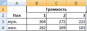
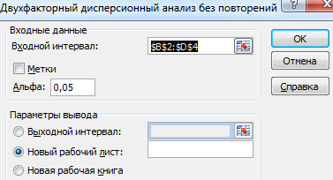
1. We open “Data Analysis”, in the list you need to find a two-way analysis of variance without repetitions.
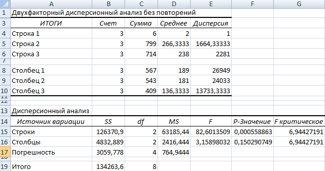
2. Input interval – cells that contain data (without a header). We display the results on a new sheet and click “OK”.

The F value is greater than the F-critical, which means that the floor affects the speed of reaction to sound.

Conclusion

In this article, sensitivity analysis in an Excel spreadsheet was discussed in detail, so that each user will be able to understand the methods of its application.