Links in Excel – absolute, relative and mixed. Errors when working with relative links in Excel

To facilitate calculations using formulas in automatic mode, references to cells are used. Depending on the type of writing, they are divided into three main types:

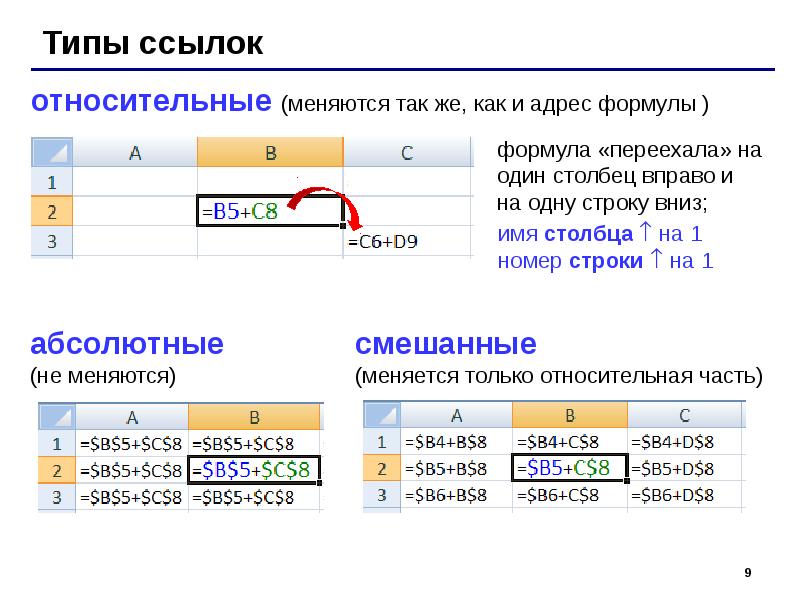
1. Relative links. Used for simple calculations. Copying a formula entails changing the coordinates.
2. Absolute links. If you need to produce more complex calculations, this option is suitable. For fixing use the symbol “$”. Example: $A$1.
3. mixed links. This type of addressing is used in calculations when it is necessary to fix a column or line separately. Example: $A1 or A$1.

If it is necessary to copy the data of the entered formula, references with absolute and mixed addressing are used. The article will reveal with examples how calculations are made using various types of links.

Relative cell reference in Excel

This is a set of characters that define the location of a cell. Links in the program are automatically written with relative addressing. For example: A1, A2, B1, B2. Moving to a different row or column changes the characters in the formula. For example, starting position A1. Moving horizontally changes the letter to B1, C1, D1, etc. In the same way, changes occur when moving along a vertical line, only in this case the number changes – A2, A3, A4, etc. If it is necessary to duplicate a calculation of the same type in an adjacent cell, a calculation is performed using a relative reference. To use this feature, follow a few steps:

1. As soon as the data is entered into the cell, move the cursor and click with the mouse. Highlighting with a green rectangle indicates the activation of the cell and the readiness for further work.
2. By pressing the key combination Ctrl + C, we copy the contents to the clipboard.
3. We activate the cell into which you want to transfer data or a previously written formula.
4. By pressing the combination Ctrl + V we transfer the data saved in the system clipboard.

Expert advice! To carry out the same type of calculations in the table, use a life hack. Select the cell containing the previously entered formula. Hovering the cursor over a small square that appears in the bottom right corner, and holding the left mouse button, drag to the bottom row or extreme column, depending on the action performed. By releasing the mouse button, the calculation will be performed automatically. This tool is called the auto fill marker.

Relative link example

To make it clearer, consider an example of a calculation using a formula with a relative reference. Suppose the owner of a sports store after a year of work needs to calculate the profit from sales.

The order of actions:

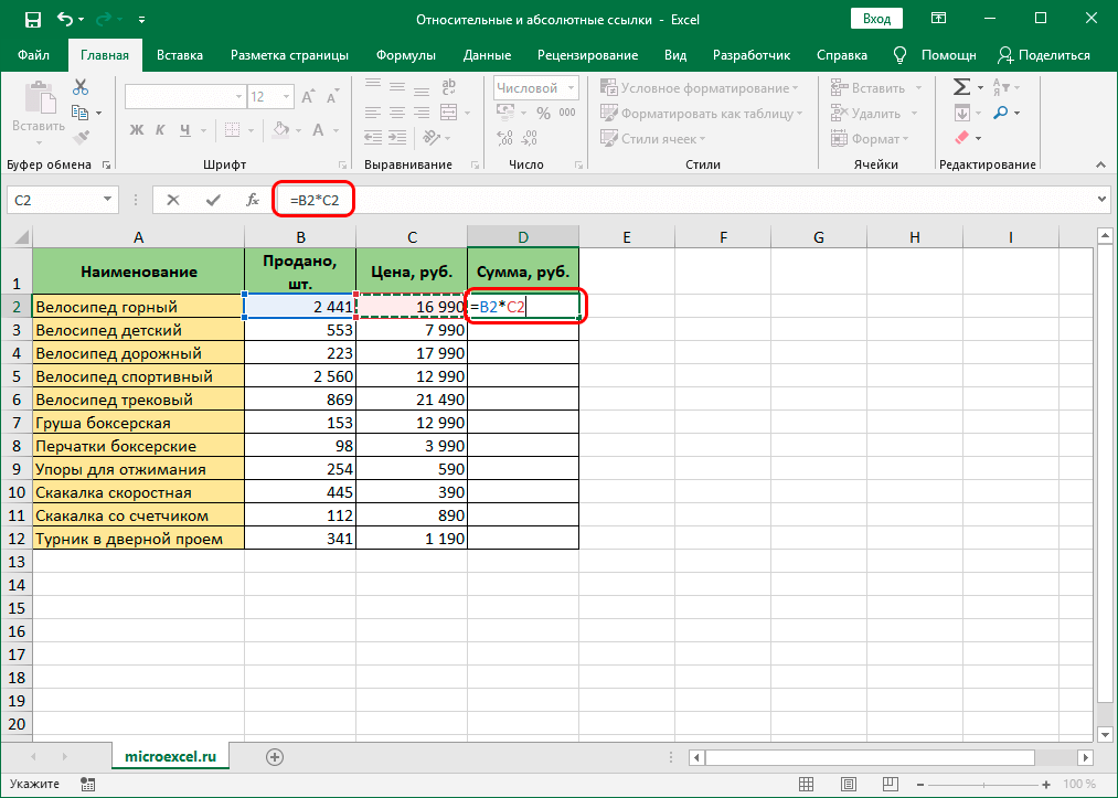
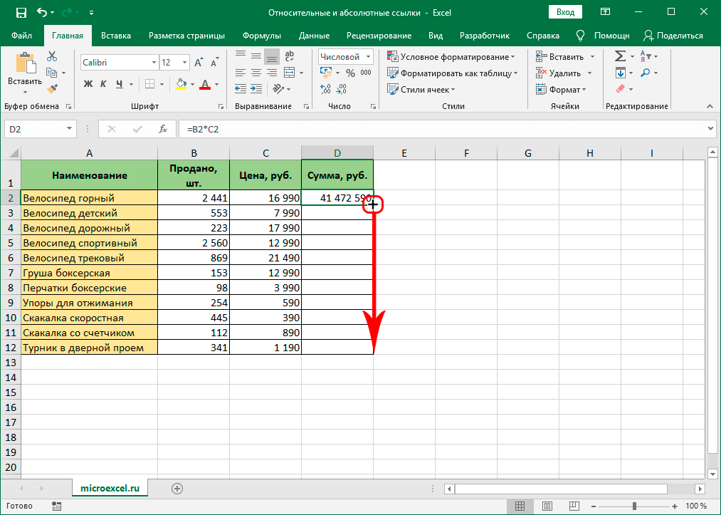
1. The example shows that columns B and C were used to fill in the quantity of goods sold and its price. Accordingly, to write the formula and get the answer, select column D. The formula looks like this: = B2 *C

Pay attention! To facilitate the process of writing a formula, use a little trick. Put the “=” sign, click on the quantity of goods sold, set the “*” sign and click on the price of the product. The formula after the equal sign will be written automatically.

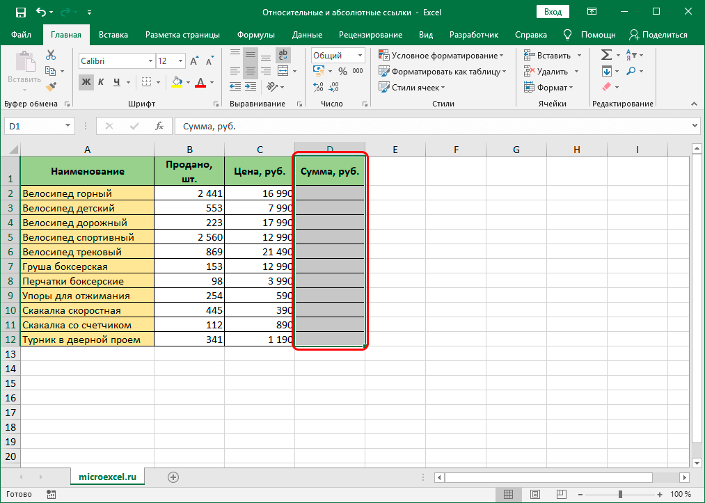
2. For the final answer, press “Enter”. Next, you need to calculate the total amount of profit received from other types of products. Well, if the number of lines is not large, then all manipulations can be performed manually. To fill in a large number of rows at the same time in Excel, there is one useful function that makes it possible to transfer the formula to other cells.
3. Move the cursor over the lower right corner of the rectangle with the formula or the finished result. The appearance of a black cross serves as a signal that the cursor can be dragged down. Thus, an automatic calculation of the profit received for each product separately is made.
4. By releasing the pressed mouse button, we get the correct results in all lines.

By clicking on cell D3, you can see that the cell coordinates have been automatically changed, and now look like this: =B3 *C3. It follows that the links were relative.

Possible errors when working with relative links

Undoubtedly, this Excel function greatly simplifies the calculations, but in some cases difficulties may arise. Let’s consider a simple example of calculating the profit coefficient of each item of goods:

1. Create a table and fill in: A – product name; B – quantity sold; C – cost; D is the amount received. Suppose there are only 11 items in the assortment. Therefore, taking into account the description of the columns, 12 lines are filled and the total amount of profit is D
2. Click on cell E2 and enter =D2/D13.
3. After pressing the “Enter” button, the coefficient of the relative share of sales of the first item appears.
4. Stretch the column down and wait for the result. However, the system gives the error “#DIV/0!”

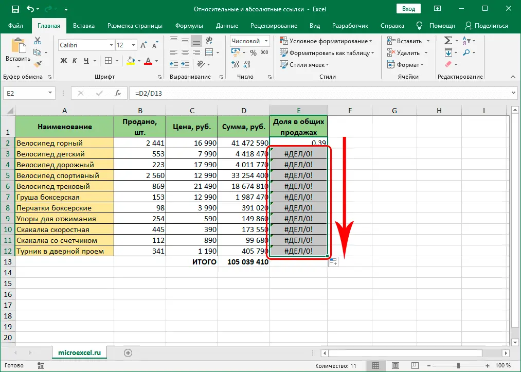
The reason for the error is the use of a relative reference for calculations. As a result of copying the formula, the coordinates change. That is, for E3, the formula will look like this =D3/D13. Because cell D13 is not filled and theoretically has a zero value, the program will give an error with the information that division by zero is impossible.

Important! To correct the error, it is necessary to write the formula in such a way that the D13 coordinates are fixed. Relative addressing has no such functionality. To do this, there is another type of links – absolute. 

How do you make an absolute link in Excel

Thanks to the use of the $ symbol, it became possible to fix the cell coordinates. How this works, we will consider further. Since the program uses relative addressing by default, accordingly, to make it absolute, you will need to perform a number of actions. Let’s analyze the solution to the error “How to find the coefficient from the sale of several items of goods”, performing the calculation using absolute addressing:

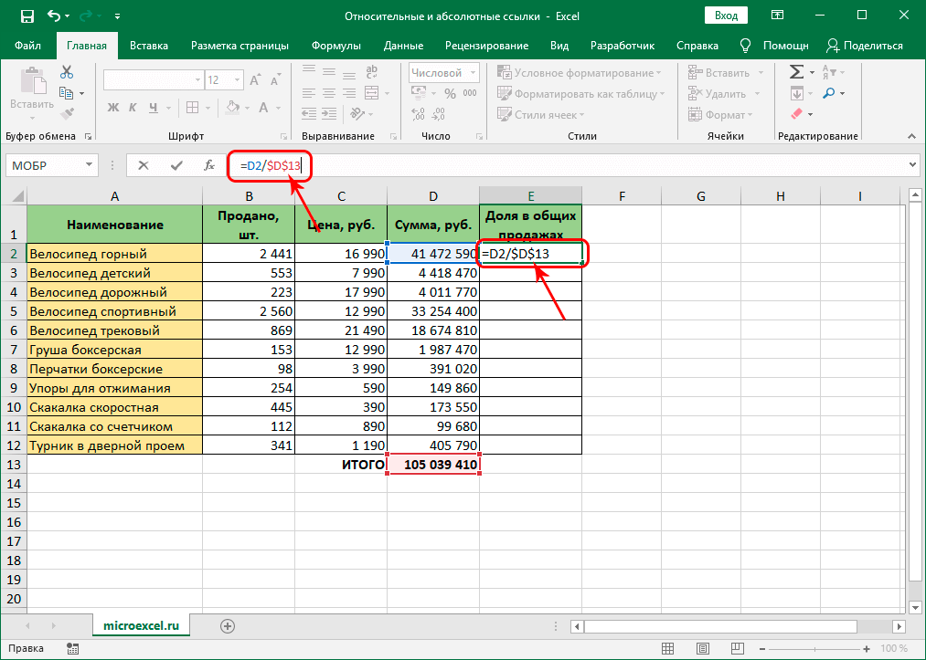
1. Click on E2 and enter the coordinates of the link =D2/D13. Since the link is relative, a symbol must be set to fix the data.
2. Fix the coordinates of cell D To perform this action, precede the letter indicating the column and the row number by placing a “$” sign.

Expert advice! To facilitate the task of entering, it is enough to activate the cell for editing the formula and press the F4 key several times. Until you get satisfactory values. The correct formula is as follows: =D2/$D$13.

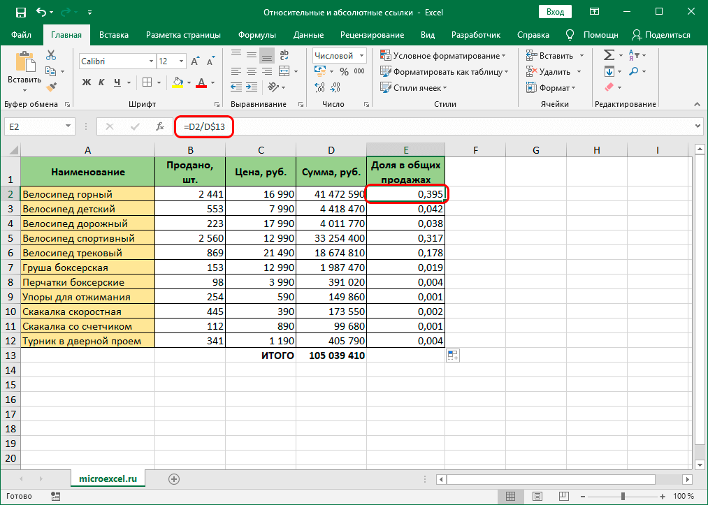
3. Press the “Enter” button. As a result of the performed actions, the correct result should appear.
4. Drag the marker to the bottom line to copy the formula.

Due to the use of absolute addressing in the calculations, the final results in the remaining rows will be correct.

How to put a mixed link in Excel

For formula calculations, not only relative and absolute references are used, but also mixed ones. Their distinctive feature is that they fix one of the coordinates.

• For example, to change the position of a line, you must write the $ sign in front of the letter designation.
• On the contrary, if the dollar sign is written after the letter designation, then the indicators in the line will remain unchanged.

From this it follows that in order to solve the previous problem with determining the coefficient of sales of goods using mixed addressing, it is necessary to fix the line number. That is, the $ sign is placed after the column letter, because its coordinates do not change even in a relative reference. Let’s take an example:

1. For accurate calculations, enter =D1/$D$3 and press “Enter”. The program gives the exact answer.
2. To move the formula to subsequent cells down the column and get accurate results, drag the handle to the bottom cell.
3. As a result, the program will give the correct calculations.

Attention! If you set the $ sign in front of the letter, then Excel will give an error “#DIV/0!”, which will mean that this operation cannot be performed.

“SuperAbsolute” addressing

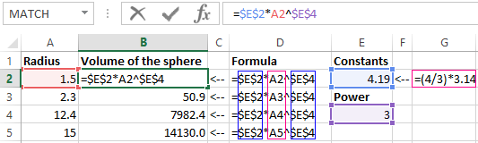
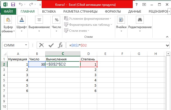
In the end, let’s look at another example of an absolute link – “SuperAbsolute” addressing. What are its features and differences. Take the approximate number 30 and enter it in cell B2. It is this number that will be the main one, it is necessary to perform a series of actions with it, for example, to raise it to a power.

1. For the correct execution of all actions, enter the following formula in column C: =$B$2^$D2. In column D we enter the value of the degrees.

2. After pressing the “Enter” button and activating the formula, we stretch the marker down the column.
3. We get the correct results.

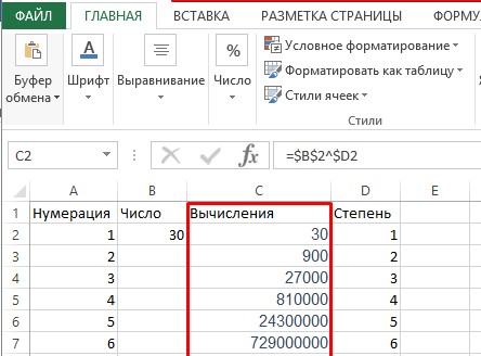
The bottom line is that all the actions performed referred to one fixed cell B2, therefore:

• Copying a formula from cell C3 to cell E3, F3, or H3 will not change the result. It will remain unchanged – 900.
• If you need to insert a new column, the coordinates of the cell with the formula will change, but the result will also remain unchanged.

This is the peculiarity of the “SuperAbsolute” link: if you need to move the result will not change. However, there are situations when data is inserted from third-party sources. Thus, the columns are shifted to the side, and the data is set in the old way in column B2. What happens in this case? When mixed, the formula changes according to the action performed, that is, it will no longer point to B2, but to C2. But since the insertion was made in B2, the final result will be wrong.

Reference! To be able to insert macros from third-party sources, you need to enable developer settings (they are disabled by default). To do this, go to Options, open the ribbon settings and check the box in the right column opposite “Developer”. After that, access to many functions that were previously hidden from the eyes of the average user will open.

This begs the question: is it possible to modify the formula from cell C2 so that the original number is collected from cell B, despite the insertion of new data columns? To ensure that changes in the table do not affect the determination of the total when installing data from third-party sources, you must perform the following steps:

1. Instead of the coordinates of cell B2, enter the following indicators: =INDIRECT(“B2”). As a result, after moving the formulating composition will look like this: =INDIRECT(“B2”)^$E2.
2. Thanks to this function, the link always points to the square with coordinates B2, regardless of whether columns are added or removed in the table.

It must be understood that a cell that does not contain any data always shows the value “0”.

Conclusion

Thanks to the use of three varieties of the described links, a lot of opportunities appear that make it easier to work with calculations in Excel. Therefore, before you start working with formulas, first read the links and the rules for their installation.