How to remove a filter in Excel

Filtering data in Excel is necessary to make it easier to work with tables and large amounts of information. So, for example, a significant part can be hidden from the user, and when the filter is activated, display the information that is needed at the moment. In some cases, when the table was created incorrectly, or due to user inexperience, it becomes necessary to remove the filter in individual columns or on the sheet completely. How exactly this is done, we will analyze in the article.

Table creation examples

Before proceeding to remove the filter, first consider the options for enabling it in an Excel spreadsheet:

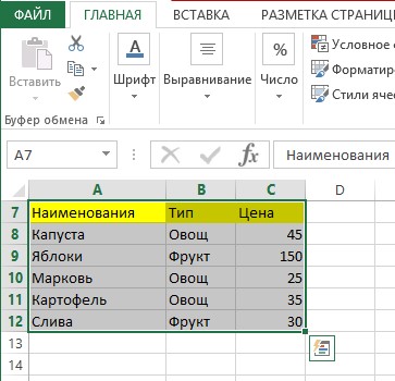
• Manual data entry. Fill in the rows and columns with the necessary information. After that, we highlight the addressing of the table location, including the headers. Go to the “Data” tab at the top of the tools. We find the “Filter” (it is displayed in the form of a funnel) and click on it with LMB. The filter in the top headers should be activated.

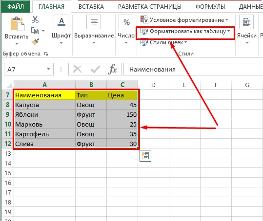
• Automatic activation of filtering. In this case, the table is also pre-filled, after which in the “Styles” tab we find the activation of the “Filter as table” line. There should be an automatic placement of filters in the subheadings of the table.

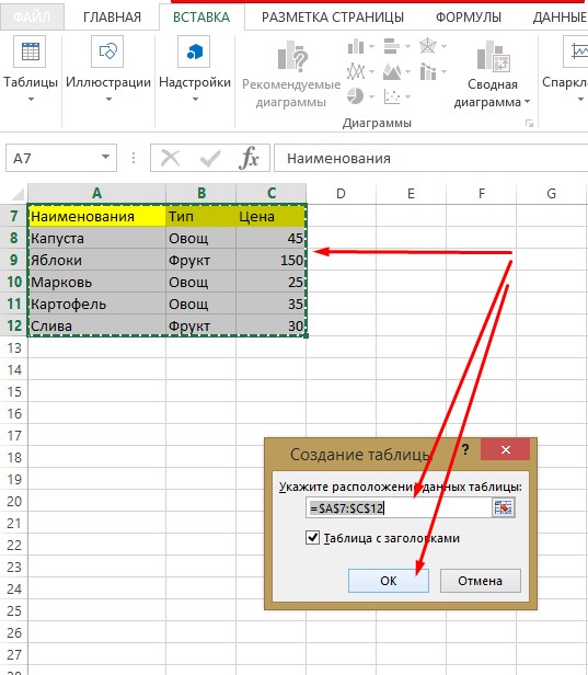
In the second case, you need to go to the “Insert” tab and find the “Table” tool, click on it with LMB and select “Table” from the following three options.

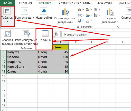
In the next interface window that opens, addressing of the created table will be displayed. It remains only to confirm it, and the filters in the subheadings will turn on automatically.

Expert advice! Before saving the completed table, make sure that the data is entered correctly and that filters are enabled.

Examples of working with a filter in Excel

Let’s leave for consideration the same sample table created earlier for three columns.

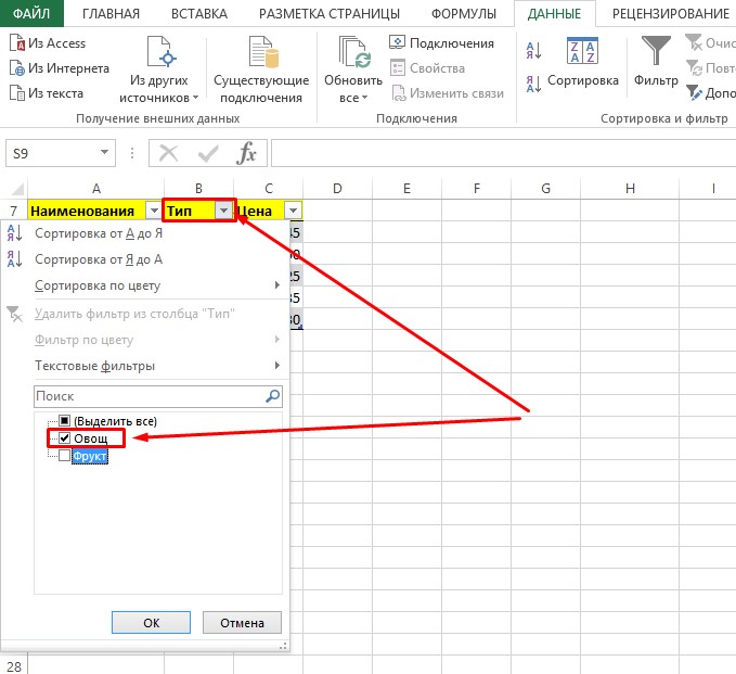
• Select the column where you want to make adjustments. By clicking on the arrow in the top cell, you can see the list. To remove one of the values ​​or names, uncheck the box next to it.
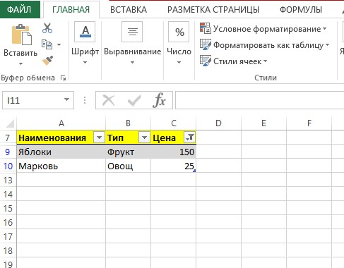
• For example, we need only vegetables to remain in the table. In the window that opens, uncheck the “fruits” box, and leave the vegetables active. Agree by clicking on the “OK” button.

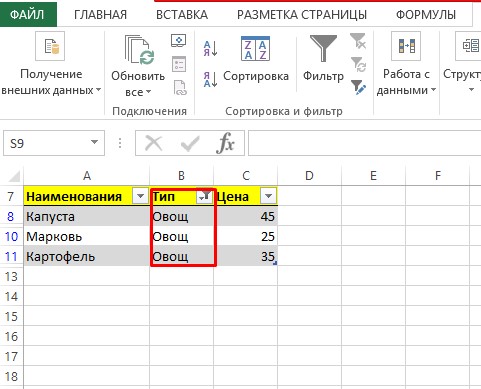
• After activation, the list will look like this:

Consider another example of how the filter works:

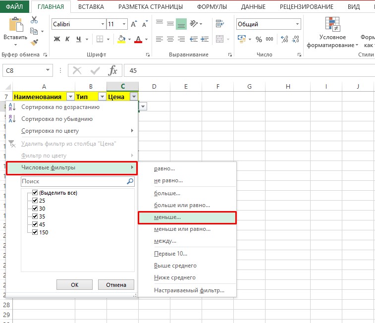
• The table is divided into three columns, and the last one contains prices for each type of product. It needs to be corrected. Let’s say we need to filter out products whose price is lower than the value “45”.
• Click on the filter icon in the selected cell. Since the column is filled with numeric values, you can see in the window that the “Numeric filters” line is in the active state.
• By hovering over it, we open a new tab with various options for filtering the digital table. In it, select the value “less”.

• Next, enter the number “45” or select by opening a list of numbers in a custom autofilter.

Attention! Entering values ​​”less than 45″, you need to understand that all prices below this figure will be hidden by the filter, including the value “45”.

Also, with the help of this function, prices are filtered in a certain digital range. To do this, in the custom autofilter, you must activate the “OR” button. Then set the value “less” at the top, and “greater” at the bottom. In the lines of the interface on the right, the necessary parameters of the price range are set, which must be left. For example, less than 30 and more than 45. As a result, the table will store the numerical values ​​25 and 150.

The possibilities for filtering informational data are actually extensive. In addition to the above examples, you can adjust the data by the color of the cells, by the first letters of the names and other values. Now that we have made a general acquaintance with the methods of creating filters and the principles of working with them, let’s move on to the removal methods.

Removing a column filter

1. First, we find the saved file with the table on our computer and double-click LMB to open it in the Excel application. On the sheet with the table, you can see that the filter is in the active state in the “Prices” column.

Expert advice! To make it easier to find the file on your computer, use the “Search” window, which is located in the “Start” menu. Enter the name of the file and press the “Enter” button on the computer keyboard.

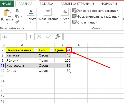
2. Click on the down arrow icon.
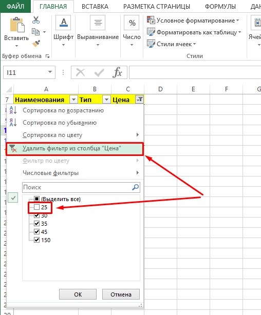
3. In the dialog box that opens, you can see that the checkmark opposite the number “25” is unchecked. If active filtering was removed only in one place, then the easiest way is to set the checkbox back and click on the “OK” button.
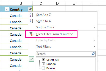
4. Otherwise, the filter must be disabled. To do this, in the same window, you need to find the line “Remove filter from the column “…”” and click on it with LMB. An automatic shutdown will occur, and all previously entered data will be displayed in full.

Removing a filter from an entire sheet

Sometimes situations may arise when it becomes necessary to remove a filter in the entire table. To do this, you will need to perform the following steps:

1. Open the saved data file in Excel.
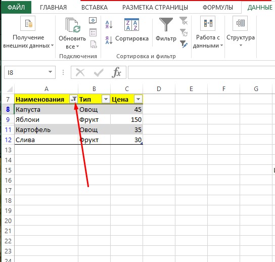
2. Find one or more columns where the filter is activated. In this case, it is the Names column.

3. Click on any place in the table or select it completely.
4. At the top, find “Data” and activate it with LMB.

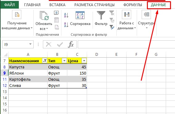
5. Find “Filter”. Opposite the column are three symbols in the form of a funnel with different modes. Click on the function button “Clear” with the funnel displayed and the red crosshair.
6. Next, active filters will be disabled for the entire table.

Conclusion

Filtering elements and values ​​in a table makes working in Excel a lot easier, but, unfortunately, a person is prone to make mistakes. In this case, the multifunctional Excel program comes to the rescue, which will help sort the data and remove unnecessary previously entered filters while preserving the original data. This feature is especially useful when filling large tables.