


Looking at a newly created chart in Excel, it is not always easy to immediately understand the trend of the data. Some charts are made up of thousands of data points. Sometimes you can tell by eye which direction the data is changing over time, other times you’ll need to resort to some Excel tools to determine what’s going on. This can be done using a trend line and a moving average line. Most often, in order to determine in which direction the data is developing, a trend line is used in the chart. To automatically calculate such a line and add it to an Excel chart, you need to take the following steps:
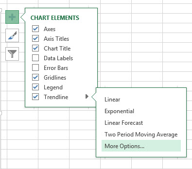
- In Excel 2013, click anywhere in the chart and then click the symbol icon plus (+) next to the diagram to open the menu Chart elements (Chart elements). Another option: click the button Add Chart Element (Add Chart Elements), which is located in the section Chart layouts (Chart Layouts) tab Constructor (Design).
- Check the box The trend line (Trendline).
- To set the type of trendline, click the arrow pointing to the right and select one of the options (linear, exponential, linear forecast, moving average, etc.).
The most commonly used are the usual linear trend and the moving average line. Linear trend – this is a straight line located in such a way that the distance from it to any of the points on the graph is minimal. This line is useful when there is confidence that subsequent data will follow the same pattern.
Very helpful moving average line at several points. Such a line, unlike a linear trend, shows the average trend for a given number of points on the chart, which can be changed. A moving average line is used when the formula providing data for plotting changes over time and the trend needs to be plotted over only a few previous points. To draw such a line, follow steps 1 and 2 from above, and then do this:
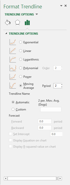
- Click the right arrow in the row The trend line (Trendline) and select an option moving average (Moving average).
- Do steps 1 and 2 from the previous example again and press More options (More options).

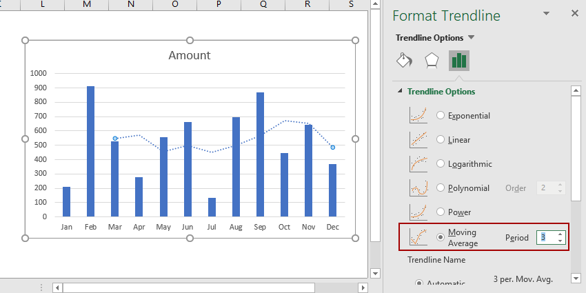
- In the opened panel Trendline Format (Format Trendline) make sure the checkbox is checked Linear filtering (Moving Average).
- To the right of the parameter Linear filtering (Moving Average) is the field Points (Period). This sets the number of points to be used to calculate the average values to plot the trend line. Set the number of points, which, in your opinion, will be optimal. For example, if you think that a certain trend in the data remains unchanged only for the last 4 points, then enter the number 4 in this field.
Trendlines in Excel is a great way to get more information about the dataset you have and how it changes over time. Linear trend and moving average are two types of trend lines that are most common and useful for business.