Horizontal column filtering in Excel

If you are not quite a novice user, then you must have already noticed that 99% of everything in Excel is designed to work with vertical tables, where parameters or attributes (fields) go through the columns, and information about objects or events is located in the lines . Pivot tables, subtotals, copying formulas with a double click – everything is tailored specifically for this data format.

However, there are no rules without exceptions and with a fairly regular frequency I am asked what to do if a table with a horizontal semantic orientation, or a table where rows and columns have the same weight in meaning, came across in the work:

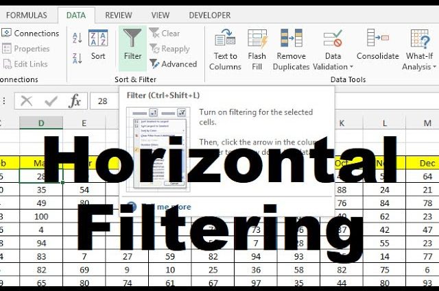
And if Excel still knows how to sort horizontally (with the command Data – Sort – Options – Sort columns), then the situation with filtering is worse – there are simply no built-in tools for filtering columns, not rows in Excel. So, if you are faced with such a task, you will have to come up with workarounds of varying degrees of complexity.

Method 1. New FILTER function

If you’re on the new version of Excel 2021 or an Excel 365 subscription, you can take advantage of the newly introduced feature FILTER (FILTER), which can filter the source data not only by rows, but also by columns. To work, this function requires an auxiliary horizontal one-dimensional array-row, where each value (TRUE or FALSE) determines whether we show or, conversely, hide the next column in the table.

Let’s add the following line above our table and write the status of each column in it:

• Let’s say we always want to display the first and last columns (headers and totals), so for them in the first and last cells of the array we set the value = TRUE.
• For the remaining columns, the contents of the corresponding cells will be a formula that checks the condition we need using functions И (AND) or OR (OR). For example, that the total is in the range from 300 to 500.

After that, it remains only to use the function FILTER to select columns above which our auxiliary array has a TRUE value:

Similarly, you can filter columns by a given list. In this case, the function will help COUNTIF (COUNTIF), which checks the number of occurrences of the next column name from the table header in the allowed list:

Method 2. Pivot table instead of the usual one

Currently, Excel has built-in horizontal filtering by columns only in pivot tables, so if we manage to convert our original table into a pivot table, we can use this built-in functionality. To do this, our source table must satisfy the following conditions:

• have a “correct” one-line header line without empty and merged cells – otherwise it will not work to build a pivot table;
• do not contain duplicates in the labels of rows and columns – they will “collapse” in the summary into a list of only unique values;
• contain only numbers in the range of values ​​(at the intersection of rows and columns), because the pivot table will definitely apply some kind of aggregating function to them (sum, average, etc.) and this will not work with the text

If all these conditions are met, then in order to build a pivot table that looks like our original table, it (the original one) will need to be expanded from the crosstab into a flat one (normalized). And the easiest way to do this is with the Power Query add-in, a powerful data transformation tool built into Excel since 2016. 

These are:

1. Let’s convert the table into a “smart” dynamic command Home – Format as a table (Home — Format as Table).
2. Loading into Power Query with the command Data – From Table / Range (Data – From Table / Range).
3. We filter the line with the totals (the summary will have its own totals).
4. Right-click on the first column heading and select Uncollapse other columns (Unpivot Other Columns). All non-selected columns are converted into two – the name of the employee and the value of his indicator.
5. Filtering the column with the totals that went into the column Attribute.
6. We build a pivot table according to the resulting flat (normalized) table with the command Home — Close and Load — Close and Load in… (Home — Close & Load — Close & Load to…).

Now you can use the ability to filter columns available in pivot tables – the usual checkmarks in front of the names and items Signature Filters (Label Filters) or Filters by value (Value Filters):

And of course, when changing the data, you will need to update our query and the summary with a keyboard shortcut Ctrl+Alt+F5 or team Data – Refresh All (Data — Refresh All).

Method 3. Macro in VBA

All the previous methods, as you can easily see, are not exactly filtering – we do not hide the columns in the original list, but form a new table with a given set of columns from the original one. If it is required to filter (hide) the columns in the source data, then a fundamentally different approach is needed, namely, a macro.

Suppose we want to filter columns on the fly where the name of the manager in the table header satisfies the mask specified in the yellow cell A4, for example, starts with the letter “A” (that is, get “Anna” and “Arthur” as a result). 

As in the first method, we first implement an auxiliary range-row, where in each cell our criterion will be checked by a formula and the logical values ​​TRUE or FALSE will be displayed for visible and hidden columns, respectively:

Then let’s add a simple macro. Right-click on the sheet tab and select command Source (Source code). Copy and paste the following VBA code into the window that opens:

Private Sub Worksheet_Change(ByVal Target As Range)      If Target.Address = "$A$4" Then          For Each cell In Range("D2:O2")              If cell = True Then                  cell.EntireColumn.Hidden = False              Else                  cell.EntireColumn.Hidden = True              End If          Next cell      End If  End Sub  

Its logic is as follows:

• In general, this is an event handler Worksheet_Change, i.e. this macro will automatically run on any change to any cell on the current sheet.
• The reference to the changed cell will always be in the variable Target.
• First, we check that the user has changed exactly the cell with the criterion (A4) – this is done by the operator if.
• Then the cycle starts For Each… to iterate over gray cells (D2:O2) with TRUE / FALSE indicator values ​​for each column.
• If the value of the next gray cell is TRUE (true), then the column is not hidden, otherwise we hide it (property Hidden).

•  Dynamic array functions from Office 365: FILTER, SORT, and UNIC
• Pivot table with multiline header using Power Query
• What are macros, how to create and use them