Circular reference in Excel. How to find and delete – 2 ways

In most cases, circular references are perceived by users as erroneous expressions. This is due to the fact that the program itself is overloaded from their presence, warning about this with a special alert. To remove unnecessary load from software processes and eliminate conflict situations between cells, it is necessary to find problem areas and remove them.

What is a circular reference

A circular reference is an expression that, through formulas located in other cells, refers to the very beginning of the expression. At the same time, in this chain there can be a huge number of links, from which a vicious circle is formed. Most often, this is an erroneous expression that overloads the system, prevents the program from working correctly. However, in some situations, users deliberately add circular references in order to perform certain computational operations.

If a circular reference is a mistake that the user made by accident when filling out a table, introducing certain functions, formulas, you need to find it and delete it. In this case, there are several effective ways. It is worth considering in detail the 2 most simple and proven in practice.

Important! Thinking about whether there are circular references in the table or not is not necessary. If such conflict situations are present, modern versions of Excel immediately notify the user about this with a warning window with relevant information.

Visual search

The simplest search method, which is suitable when checking small tables. Procedure:

1. When a warning window appears, close it by pressing the OK button.
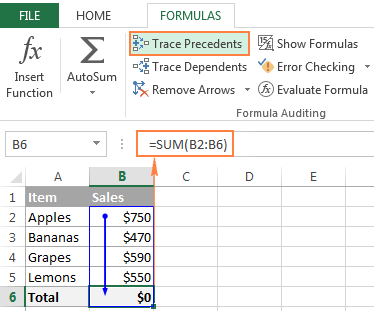
2. The program will automatically designate those cells between which a conflict situation has arisen. They will be highlighted with a special trace arrow.

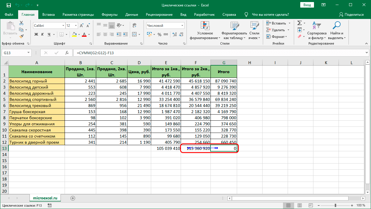
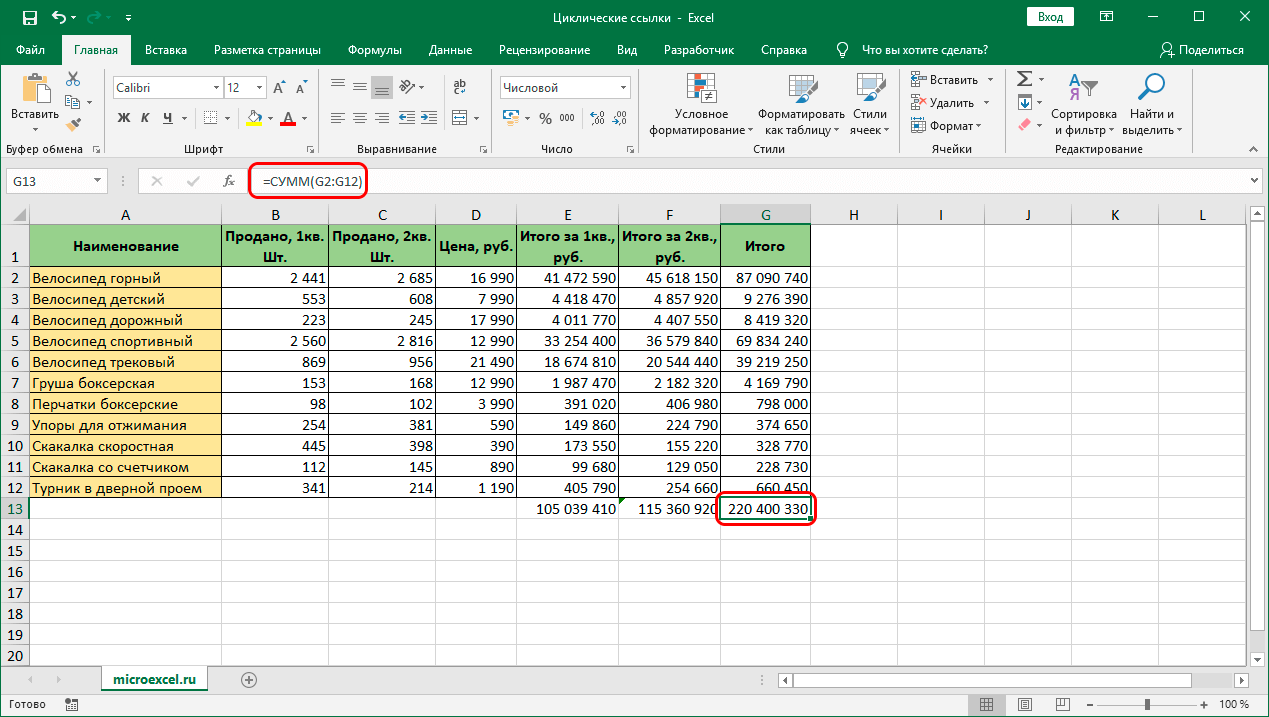
3. To remove the cyclicity, you need to go to the indicated cell and correct the formula. To do this, it is necessary to remove the coordinates of the conflict cell from the general formula.
4. It remains to move the mouse cursor to any free cell in the table, click LMB. The circular reference will be removed.

Using the program tools

In cases where the trace arrows do not point to problem areas in the table, you must use the built-in Excel tools to find and remove circular references. Procedure:

1. First of all, you need to close the warning window.
2. Go to the “Formulas” tab on the main toolbar.
3. Go to the Formula Dependencies section.
4. Find the “Check for Errors” button. If the program window is in a compressed format, this button will be marked with an exclamation point. Next to it should be a small triangle that points down. Click on it to bring up a list of commands.

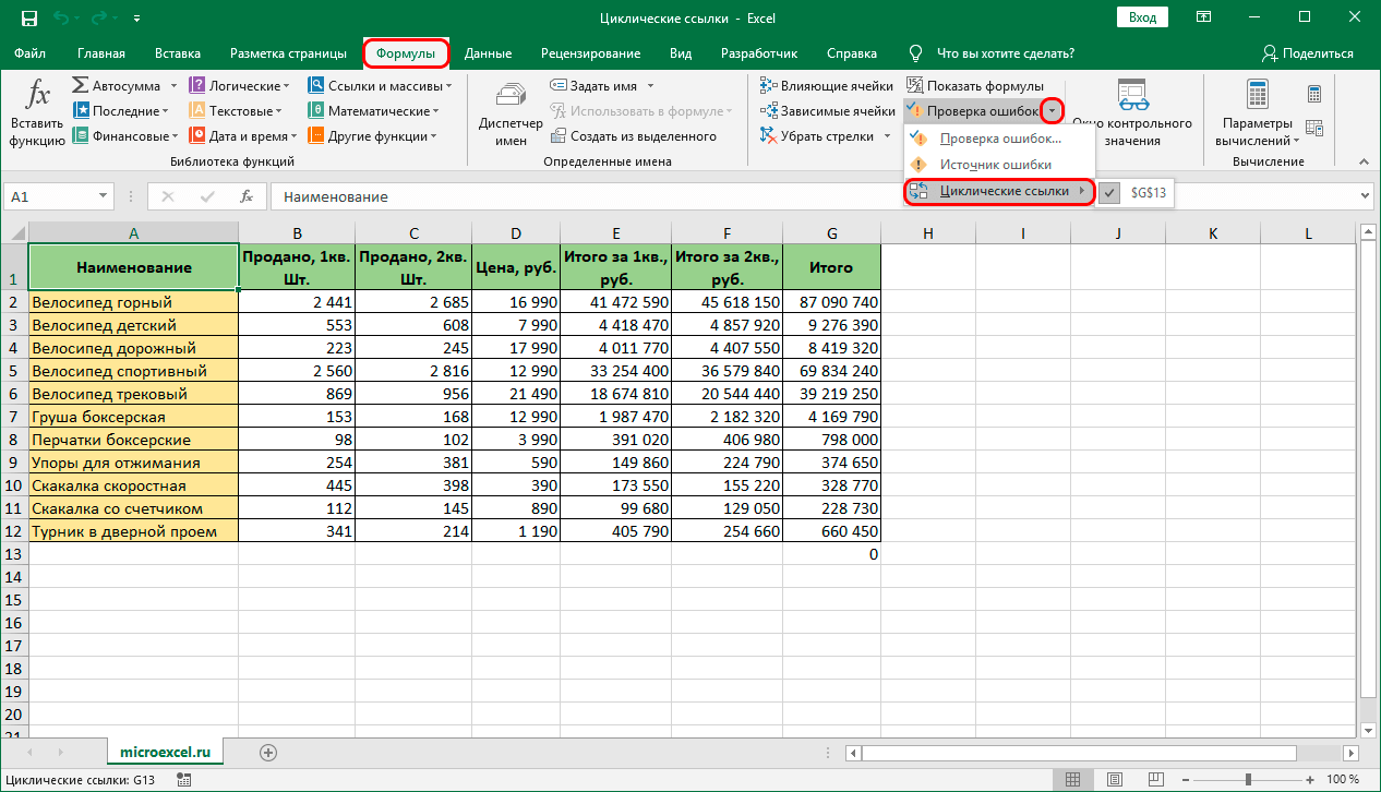
5. Select “Circular Links” from the list.
6. After completing all the steps described above, the user will see a complete list with cells that contain circular references. In order to understand exactly where this cell is located, you need to find it in the list, click on it with the left mouse button. The program will automatically redirect the user to the place where the conflict occurred.
7. Next, you need to fix the error for each problematic cell, as described in the first method. When conflicting coordinates are removed from all formulas that are in the error list, a final check must be performed. To do this, next to the “Check for errors” button, you need to open a list of commands. If the “Circular Links” item is not shown as active, there are no errors.

Disabling locking and creating circular references

Now that you’ve figured out how to find and fix circular references in Excel spreadsheets, it’s time to look at situations where these expressions can be used to your advantage. However, before that, you need to learn how to disable automatic blocking of such links.

Most often, circular references are deliberately used during the construction of economic models, to perform iterative calculations. However, even if such an expression is used consciously, the program will still automatically block it. To run the expression, you must disable the lock. To do this, you need to perform several actions:

1. Go to the “File” tab on the main panel.
2. Select “Settings”.
3. The Excel setup window should appear before the user. From the menu on the left, select the “Formulas” tab.
4. Go to the Calculation Options section. Check the box next to the “Enable iterative calculations” function. In addition to this, in the free fields just below you can set the maximum number of such calculations, the permissible error.

Important! It is better not to change the maximum number of iterative calculations unless absolutely necessary. If there are too many of them, the program will be overloaded, there may be failures with its work.

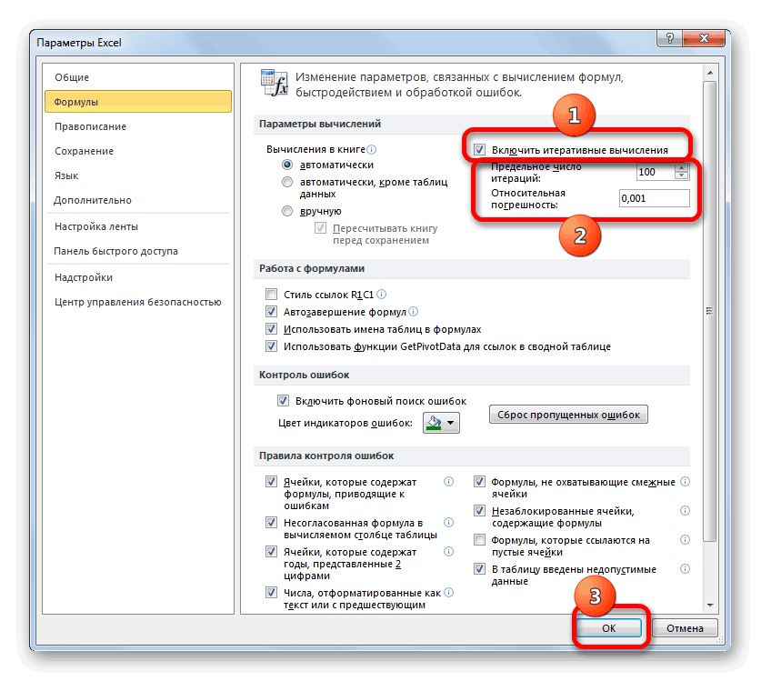
5. For the changes to take effect, you must click on the “OK” button. After that, the program will no longer automatically block calculations in cells that are linked by circular references.

The easiest way to create a circular link is to select any cell in the table, enter the “=” sign into it, immediately after which add the coordinates of the same cell. To complicate the task, to extend the circular reference to several cells, you need to follow the following procedure:

1. In cell A1 add the number “2”.
2. In cell B1, enter the value “=C1”.
3. In cell C1 add the formula “=A1”.
4. It remains to return to the very first cell, through it refer to cell B1. After that, the chain of 3 cells will close.

Conclusion

Finding circular references in an Excel spreadsheet is easy enough. This task is greatly simplified by the automatic notification of the program itself about the presence of conflicting expressions. After that, it remains only to use one of the two methods described above to get rid of errors.