


Most of those who have ever built graphs in Microsoft Excel or PowerPoint have noticed an unusual and funny type of charts – bubble charts. Many have seen them in other people’s files or presentations. However, in 99 cases out of 100, when trying to build such a diagram for the first time, users encounter a number of non-obvious difficulties. Usually, Excel either refuses to create it at all, or creates it, but in a completely incomprehensible form, without signatures and clarity.
Let’s look into this topic.
What is a bubble chart
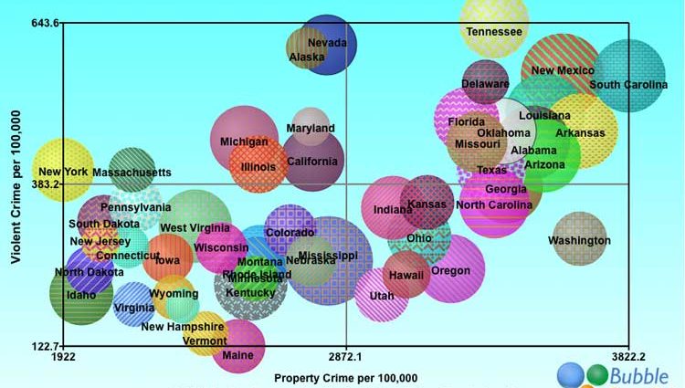
A bubble chart is a specific type of chart that can display XNUMXD data in XNUMXD space. For example, consider this chart that displays statistics by country from the well-known chart designer site http://www.gapminder.org/ :

You can download the full size PDF from here http://www.gapminder.org/downloads/gapminder-world-map/
The horizontal x-axis represents the average annual per capita income in USD. The vertical y-axis represents life expectancy in years. The size (diameter or area) of each bubble is proportional to the population of each country. Thus, it is possible to display three-dimensional information on one flat chart.
An additional informational load is also carried by the color, which reflects the regional affiliation of each country to a particular continent.
How to build a bubble chart in Excel
The most important point in building a bubble chart is a properly prepared table with source data. Namely, the table must consist strictly of three columns in the following order (from left to right):
- Parameter for laying on the x-axis
- Parameter for y-drag
- Parameter defining the size of the bubble
Let’s take for example the following table with data on game consoles:

To build a bubble chart on it, you need to select a range C3:E8 (strictly – only orange and gray cells without a column with names) and then:
- In Excel 2007/2010 – go to the tab Insert — Group Diagrams — Others — Bubble (Insert — Chart — Bubble)
- In Excel 2003 and later, choose from the menu Insert – Chart – Bubble (Insert — Chart — Bubble)

The resulting chart will display the speed of the set-top boxes on the x-axis, the number of programs for them on the y-axis, and the market share occupied by each set-top box – as the size of a bubble:

After creating a bubble chart, it makes sense to set up labels for the axes – without the titles of the axes, it is difficult to understand which of them is plotted. In Excel 2007/2010, this can be done on the tab Layout (Layout), or in older versions of Excel, by right-clicking the chart and choosing Chart Options (Chart options) – tab Headlines (Titles).
Unfortunately, Excel does not allow you to automatically bind the color of the bubbles to the source data (as in the example above with countries), but for clarity, you can quickly format all the bubbles in different colors. To do this, right-click on any bubble, select command Data series format (Format series) from the context menu and enable the option colorful dots (Vary colors).
Problem with signatures
A common difficulty that absolutely all users face when building bubble (and scatter, by the way, too) charts is labels for bubbles. Using standard Excel tools, you can display as signatures only the X, Y values, the size of the bubble, or the name of the series (common for all). If you recall that when building a bubble chart, you did not select a column with labels, but only three columns with data X, Y and the size of the bubbles, then everything turns out to be generally logical: what is not selected cannot get into the chart itself.
There are three ways to solve the problem of signatures:
Method 1. Manually
Manually rename (change) captions for each bubble. You can simply click on the container with the caption and enter a new name from the keyboard instead of the old one. Obviously, with a large number of bubbles, this method begins to resemble masochism.
Method 2: XYChartLabeler add-in
It is not difficult to assume that other Excel users have encountered a similar problem before us. And one of them, namely the legendary Rob Bovey (God bless him) wrote and posted a free add-on to the public XYChartLabeler, which adds this missing function to Excel.
You can download the add-on here http://appspro.com/Utilities/ChartLabeler.htm
After installation, you will have a new tab (in older versions of Excel – toolbar) XY Chart Labels:

By selecting the bubbles and using the button Add Labels you can quickly and conveniently add labels to all the bubbles in the chart at once, simply by setting the range of cells with text for labels:

Method 3: Excel 2013
The new version of Microsoft Excel 2013 finally has the ability to add labels to chart data elements from any randomly selected cells. We waited 🙂
