


Contents
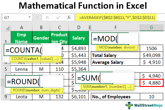
As a rule, people use only a limited number of Excel formulas, although there are a number of functions that people unfairly forget about. However, they can be of great help in solving many problems. To get acquainted with mathematical functions, you need to open the “Formulas” tab and find the “Math” item there. We will look at some of these functions because each of the possible formulas in Excel has its own practical use.
Mathematical functions of random numbers and possible combinations
These are functions that allow you to work with random numbers. I must say that there are no truly random numbers. All of them are generated according to certain patterns. Nevertheless, for solving applied problems, even a generator of not quite random numbers can be very useful. Mathematical functions that generate random numbers include BETWEEN THE CASE, SLCHIS, CHISLCOMB, FACT. Let’s look at each of them in more detail.
Function BETWEEN THE CASE
This is one of the most used features in this category. It generates a random number that fits within a certain limit. It is important to consider that if the range is too narrow, the numbers may be the same. The syntax is very simple: =RANDBETWEEN(lower value; upper value). The parameters passed by the user can be both numbers and cells that contain certain numbers. Mandatory input for each argument.
The first number in brackets is the minimum number below which the generator will not work. Accordingly, the second is the maximum number. Beyond these values, Excel will not look for a random number. The arguments can be the same, but in this case only one number will be generated.
This number is constantly changing. Each time the document is edited, the value is different.
Function SLCHIS
This function generates a random value, the boundaries of which are automatically set at the level of 0 and 1. You can use several formulas using this function, as well as use one function several times. In this case, there will be no modification of the readings.
You don’t need to pass any additional parameters to this function. Therefore, its syntax is as simple as possible: =SUM(). It is also possible to return fractional random values. To do this, you need to use the function SLCHIS. The formula will be: =RAND()*(max limit-min limit)+min limit.
If you extend the formula to all cells, then you can set any number of random numbers. To do this, you must use the autofill marker (the square in the lower left corner of the selected cell).
Function NUMBERCOMB
This function belongs to such a branch of mathematics as combinatorics. It determines the number of unique combinations for a certain number of objects in the sample. It is actively used, for example, in statistical research in the socionomic sciences. The syntax of the function is as follows: =NUMBERCOMB(set size, number of elements). Let’s look at these arguments in more detail:
- The set size is the total number of elements in the sample. It can be the number of people, goods, and so on.
- Amount of elements. This parameter denotes a link or a number indicating the total number of objects that should result. The main requirement for the value of this argument is that it must always be smaller than the previous one.
Entering all arguments is required. Among other things, they must all be positive in modality. Let’s take a small example. Let’s say we have 4 elements – ABCD. The task is as follows: to choose combinations in such a way that the numbers do not repeat. However, their location is not taken into account. That is, the program will not care if it is a combination of AB or BA.
Let’s now enter the formula we need to get these combinations: =NUMBERCOMB(4). As a result, 6 possible combinations will be displayed, consisting of different values.
INVOICE function
In mathematics, there is such a thing as factorial. This value means the number that is obtained by multiplying all natural numbers up to this number. For example, the factorial of the number 3 will be the number 6, and the factorial of the number 6 will be the number 720. The factorial is denoted by an exclamation point. And using the function FACTOR it becomes possible to find the factorial. Formula syntax: =FACT(number). The factorial corresponds to the number of possible combinations of values in the set. For example, if we have three elements, then the maximum number of combinations in this case will be 6.
Number conversion functions
Converting numbers is the performance of certain operations with them that are not related to arithmetic. For example, turning a number into Roman, returning its module. These features are implemented using the functions ABS and ROMAN. Let’s look at them in more detail.
ABS function
We remind you that the modulus is the distance to zero on the coordinate axis. If you imagine a horizontal line with numbers marked on it in increments of 1, then you can see that from the number 5 to zero and from the number -5 to zero there will be the same number of cells. This distance is called the modulus. As we can see, the modulus of -5 is 5, since it takes 5 cells to go through to get to zero.
To get the modulus of a number, you need to use the ABS function. Its syntax is very simple. It is enough to write a number in brackets, after which the value will be returned. The syntax is: =ABS(number). If you enter the formula =ABS(-4), then the result of these operations will be 4.
ROMAN function
This function converts a number in Arabic format to Roman. This formula has two arguments. The first one is mandatory, and the second one can be omitted:
- Number. This is directly a number, or a reference to a cell containing a value in this form. An important requirement is that this parameter must be greater than zero. If the number contains digits after the decimal point, then after its conversion to the Roman format, the fractional part is simply cut off.
- Format. This argument is no longer required. Specifies the presentation format. Each number corresponds to a certain appearance of the number. There are several possible options that can be used as this argument:
- 0. In this case, the value is shown in its classic form.
- 1-3 – different types of display of Roman numbers.
- 4. Lightweight way to show Roman numerals.
- Truth and Falsehood. In the first situation, the number is presented in standard form, and in the second – simplified.
SUBTOTAL function
This is a fairly complex function that gives you the ability to sum up subtotals based on the values that are passed to it as arguments. You can create this function through the standard functionality of Excel, and it is also possible to use it manually.
This is a rather difficult function to use, so we need to talk about it separately. The syntax for this function is:
- Feature number. This argument is a number between 1 and 11. This number indicates which function will be used to sum up the specified range. For example, if we need to add numbers, then we need to specify the number 9 or 109 as the first parameter.
- Link 1. This is also a required parameter that gives a link to the range taken into account for summarizing. As a rule, people use only one range.
- Link 2, 3… Next comes a certain number of links to the range.
The maximum number of arguments that this function can contain is 30 (function number + 29 references).
Important note! Nested totals are ignored. That is, if the function has already been applied in some range SUBTOTALS, it is ignored by the program.
Also note that using this function to subtotal horizontal arrays of data is not recommended as it is not designed for that. In this case, the results may be incorrect. Function SUBTOTALS often combined with an autofilter. Suppose we have such a dataset.
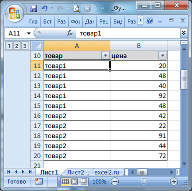
Let’s try to apply an autofilter to it and select only the cells marked as “Product1”. Next, we set the task to determine using the function SUBTOTALS the subtotal of these goods. Here we need to apply code 9 as shown in the screenshot.
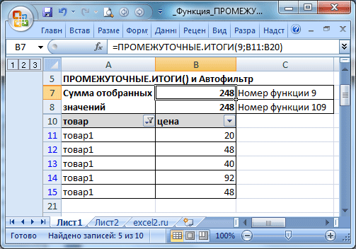
Further, the function automatically selects those rows that are not included in the filter result and does not include them in the calculations. This gives you many more options. By the way, there is a built-in Excel function called Subtotals. What is the difference between these tools? The fact is that the function automatically removes from the selection all rows that are not currently displayed. This does not take into account the code function_number.
By the way, this tool allows you to do a lot of things, and not just determine the sum of values. Here is a list of codes with functions that are used to sum up subtotals.
1 – HEART;
2 – COUNT;
3 – SCHÖTZ;
4 – MAX;
5 MINUTES;
6 – PRODUCT;
7 – STDEV;
8 – STANDOTKLONP;
9 – SUM;
10 – DISP;
11 – DISP.
You can also add 100 to these numbers and the functions will be the same. But there is one difference. The difference is that in the first case, hidden cells will not be taken into account, while in the second case they will.
Other math functions
Mathematics is a complex science that includes many formulas for a wide variety of tasks. Excel includes almost everything. Let’s look at just three of them: SIGN, Pi, PRODUCT.
SIGN function
With this function, the user can determine whether the number is positive or negative. It can be used, for example, to group clients into those who have debts in the bank and those who have not taken out a loan or repaid it at the moment.
The function syntax is as follows: =SIGN(number). We see that there is only one argument, the input of which is mandatory. After checking the number, the function returns the value -1, 0, or 1, depending on what sign it was. If the number turned out to be negative, then it will be -1, and if it is positive – 1. If zero is caught as an argument, then it is returned. The function is used in conjunction with the function IF or in any other similar case when you need to check the number.
Function Pi
The number PI is the most famous mathematical constant, which is equal to 3,14159 … Using this function, you can get a rounded version of this number to 14 decimal places. It has no arguments and has the following syntax: =PI().
Function PRODUCT
A function similar in principle to SUM, only calculates the product of all numbers passed to it as arguments. You can specify up to 255 numbers or ranges. It is important to consider that the function does not take into account text, logical and any other values that are not used in arithmetic operations. If a boolean value is used as an argument, then the value TRUE corresponds to one, and the value FALSE – zero. But it is important to understand that if there is a boolean value in the range, then the result will be wrong. The formula syntax is as follows: =PRODUCT(number 1; number 2…).
We see that numbers are given here separated by a semicolon. The required argument is one – the first number. In principle, you can not use this function with a small number of values. Then you need to consistently multiply all the numbers and cells. But when there are a lot of them, then in manual mode it will take quite a lot of time. To save it, there is a function PRODUCT.
Thus, we have a huge number of functions that are used quite rarely, but at the same time they can be of good use. Do not forget that these functions can be combined with each other. Consequently, the range of possibilities that open up is greatly expanded.