


Contents
Mathematics is the queen of sciences. And indeed so. It is impossible to do without it even in the humanities. If some activity does not require mathematical tools, it immediately loses its seriousness. The complexity is added by the need to know all these formulas. Although after people got the Excel program, there really were fewer problems in this part. Today we will analyze the basic mathematical formulas that are used in statistical calculations and database processing. And in this part, we will focus on the functions related to rounding.
First, we need to understand what rounding is in general? We know that there are two kinds of numbers: round and not. The first ones are those that end in zero. Rounding is the process of converting numbers that do not end in zero.
The second rounding option is the conversion of a fractional number into an integer. For example, we have the number 56,78. After rounding, it will become 57. There are many rounding methods provided in Excel, but let’s start by describing the standard rounding method.
- If the number ends with a digit less than 5, it is rounded down.
- If the number ends with a digit greater than 5, it is rounded up.
- If the number ends in 5, then theoretically you can round up in any direction, but in practice the number is usually reduced. But in some other areas of activity, it is customary to round this number to a lower value. There are special formulas for this in Excel.
Rounding is a very useful feature when there is no need to achieve very high precision. Previously, rounding was used much more widely because it was not possible to fit so many numbers on one sheet. Also, the presence of extra signs can significantly increase the amount of work that needs to be done, despite the fact that there is no significant increase in the return on such labor costs. Now there is no such urgent need to round the values, since the computer is able to do everything for a person. However, in some areas, rounding still occupies a significant position, since it allows you to avoid fatal errors.
In fact, you will have to round the numbers anyway, because there is no perfect accuracy even in science. By the way, because of this, the butterfly effect was discovered. It is enough to round a number with a large number of decimal places in the mathematical model, as the final value changes completely.
Due to the inaccuracy of numbers, such a thing as a statistical error appeared. True, after the advent of computers, in complex calculations, rounding in intermediate values no longer occurs as much. Only the final result rises or falls depending on what number was in the last digit. Here we need to introduce a new concept: significant digits. These are the digits that determine how accurate a certain number will be.
NONE function
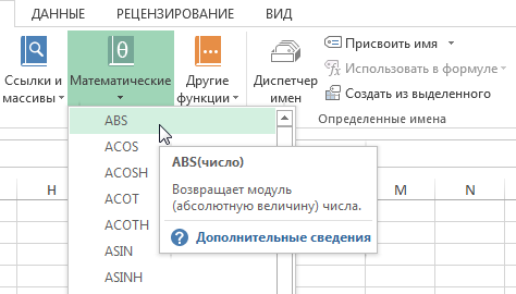
Each of the functions described in this article is located in the “Math” section, which can be found under the “Formulas” tab. Let’s start with the one that makes it possible to round a number to the nearest odd number. In practice, it works like this. If we have the number 5,85 and pass this formula through it, the number 7 will come out, because after rounding it normally turns out to be 6, but since this number is even, the value automatically increases.
The same goes for negative values. The only difference is that it will return a negative number. If the number -5,85 is passed as an argument to this function, then the result will be the number -7. The syntax of this function is very simple and contains only the number that needs to be rounded. The general formula looks like this: =ODD(number).
Function THU
The syntax is similar, except that the number will be rounded up to the nearest even number. And also, depending on the sign, a positive or negative value will be returned. So, if you pass the number 6,85, then the formula will automatically round the given value according to all the rules, after which it will find the even number closest to it and return the value. The result is 8. If you pass a value below zero, you get -8. In general, the formula is: =EVEN(number).
INT function
Allows you to determine which number will be closest when rounding a given fractional value down. The syntax is also very simple and consists of a single argument: =INTEGER(number). In practice, it looks like this. If we pass the number 5,85, then the result will be 5. That is, the part of the number after the decimal point will be omitted.
The principle of forming a negative number is approximately the same, with the only exception that the modulus is then not taken into account. Therefore, it turns out that when passing the value -5,85, the program will return the value 6.
BLOOD MAT function
This is a relatively new feature that was only introduced in Excel 2013. It determines which number is a multiple of another and rounds the first to the resulting digit. This formula is more complicated than the previous ones because it contains two arguments. Its syntax is the following: =RIGHTBOTTOM.MAT(number, [precision], [mode]). Let’s decipher these arguments:
- Number. This argument must be specified in all cases. It can contain two types of values: either a number or a cell.
- Accuracy. This is the number for which you need to specify the smallest multiple. The first argument is the number itself, which the second number must be a multiple of. If you specify the number 0 here, then the function will always return a zero value. This argument is also required.
- Mode. This argument specifies the rounding method. It can be done modulo or not.
ROCKUP.MAT
This function is very similar to the previous one, but the rounding is carried out not in the direction closer to zero, but in the direction of a larger multiple. The syntax is the same, the arguments are the same, but the final result changes. Very often people confuse the third arguments of the previous function with this one. Let’s describe the differences between them in more detail:
- If the function is used ROCKUP.MAT takes the value 0 in the third argument, then the effect of this argument will only apply to numbers below zero.
- If set in the third function argument OKRVNIZ.MAT zero value, then rounding will be carried out not towards zero, but from zero.
ROUND
Rounds the number in the first argument according to the options given in the second argument. This formula also looks for the nearest multiple, but does not provide for the ability to set the mode. The syntax for this function is: =ROUND(number, precision). The argument values are the same as in the previous example:
- Number. This is the number that will be a multiple of the second value.
- Accuracy. This is the number for which the closest multiple is being sought.
In what situations might you want to round a number to the nearest multiple? For example, to understand how many boxes are needed in order to deliver a certain amount of goods from point A to point B. Function ROUND also used to round a minus value to a negative multiple. The same applies to fractional values.
ROUND DOWN
A function that forces a number to be rounded down. As we know, the standard rounding rule is to round down if the last digit is less than 5 and up if it is more. But in practice, it may be necessary to round down, even if all mathematical laws require rounding up. Takes two arguments:
- Number. This contains either a number or a reference to a cell that contains that number.
- Number of digits. This is the degree of rounding. Passes information to the program about how many decimal places or how many digits to leave in the result of rounding. This argument accepts numeric values, where 0 is an integer. Accordingly, with each added digit, the degree of rounding increases. 1 is adding tenths to a number, 2 is adding hundredths, and so on.
You can also pass negative numbers to this argument. In this case, rounding is carried out by the digits of an integer, where -1 is rounding to tens, and so on.
KRUGLVVERH
This formula is completely similar to the previous one: it has the same syntax. The only difference is that it rounds up. Sometimes you still need to use the EVEN and ODD function if you need to round up to the top or bottom.
OTBR
This function removes the fractional part of the number. Rounding does not occur, it just remains the number that was in the integer part. The syntax of the formula is similar to the previous one, but the mechanism is different:
- Number. This is a number or a reference to a cell with a number from which you want to discard the fractional part.
- Number of digits. This argument is optional in this situation. The number in this argument specifies the number of characters to truncate.
ROUNDWOOD
This is standard mathematical rounding with a certain precision. Actually, the syntax is also standard – the number and number of digits. Both arguments are required. And similarly to the formulas described above, you can pass negative numbers as an argument with the number of digits. In this case, rounding will be carried out to tens, hundreds, thousands, and so on. We see that there are really a lot of rounding formulas. It is unlikely that all of them will be useful in life, but at least you need to understand their meaning in order to correctly read other people’s tables.
I should summarize the above with some general rounding rules to consider before introducing this function into your Excel user’s arsenal. It is highly recommended to practice with these functions and try your own different parameters and numbers in order to hit the number that contains the required number of digits. The rules themselves are:
- If the number is negative, it is turned into a number that does not have a minus sign, processed, after which -1 is added to it again. At first glance, this approach may not be logical, but rounding negative values is done in this way. For example, if we use the rounding function ROUND DOWN, then as a result of processing the number -889 we will get the number -880. First, the minus turns into a plus, after which the minus is attached again.
- If the number is positive, then the function ROUND DOWN rounds the number down, and the function KRUGLVVERH – up.
- Rules for rounding fractional numbers using a function ROUNDWOOD: If the number is greater than or equal to 0,5 (or the last decimal place is 5 or greater), then rounding up. If less than 0,5 then the number is rounded down.
- Rounding integers is carried out according to the same rules, only up to a larger digit before the decimal point (if you represent an integer as 66,000000).
- Significant digits are counted from the left side. For example, if we have a task to round the number 444555666 to three significant digits, then we will get 444000000 as a result, if the operation is carried out using the function ROUND DOWN.
Thus, in the arsenal of Excel there are many formulas that allow you to perform rounding of various types. Accordingly, they can be used in various fields. This is very handy when you need to round down to a lower value, for example. Moreover, all these formulas are very easy to use. Using them allows you to be more flexible in the calculation process and use the toolbar when you need to round a specific cell, regardless of the value, and formulas – when you need to round a specific value.