


Contents
An Excel function is a statement that allows you to automate a specific process of working with databases. They come in different types: mathematical, logical and others. They are the main feature of this program. Excel math functions are among the most commonly used. This is not surprising, since this is a program that was originally created to simplify the processing of huge amounts of numbers. There are many math functions, but here are 10 of the most useful ones. Today we are going to review them.
How to apply mathematical functions in the program?
Excel provides the ability to use more than 60 different mathematical functions, with which you can carry out all operations. There are several ways to insert a mathematical function into a cell:
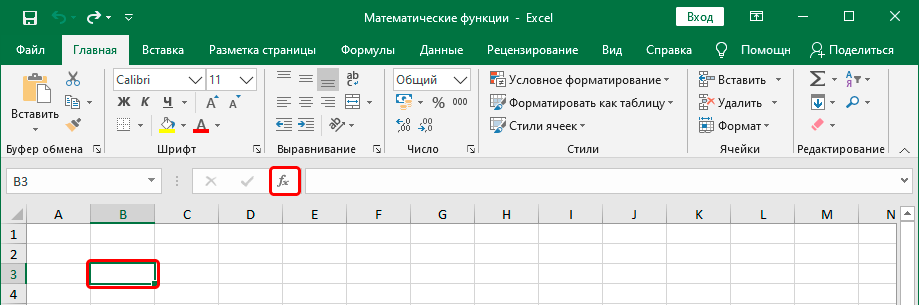
- Using the “Insert Function” button, which is located to the left of the formula entry bar. Regardless of which main menu tab is currently selected, you can use this method.

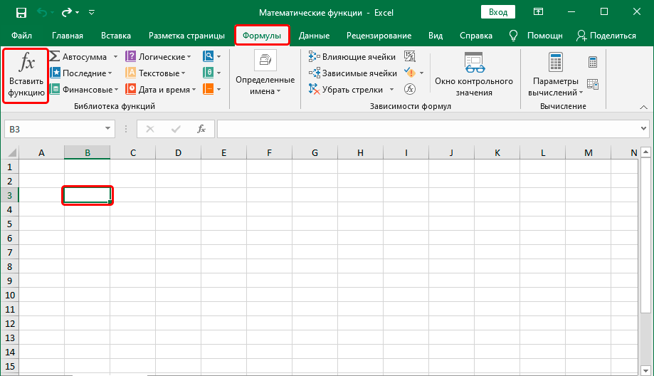
- Use the Formulas tab. There is also a button with the ability to insert a function. It is located on the very left side of the toolbar.
- Use the hot keys Shift+F3 to use the function wizard.
The latter method is the most convenient, although at first glance it is more difficult due to the need to memorize the key combination. But in the future, it can save a lot of time if you do not know which function can be used to implement a particular feature. After the function wizard is called, a dialog box will appear.
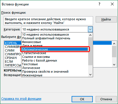
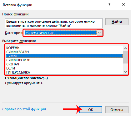
In it you can see a drop-down list with categories, and we are interested in how quick-witted readers could understand mathematical functions. Next, you need to select the one that interests us, and then confirm your actions by pressing the OK button. Also, the user can see those that are of interest to him and read their description.
Next, a window will appear with the arguments that we need to pass to the function. 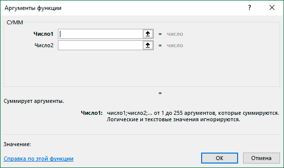
By the way, you can select mathematical functions immediately from the tape. To do this, you need the leftmost panel, click on the icon highlighted with a red square, and then select the desired function.
You can also enter the function yourself. For this, an equal sign is written, after which the name of this function is entered manually. Let’s see how this works in practice by giving specific function names.
List of mathematical functions
Now let’s list the most popular mathematical functions that are used in all possible areas of human life. This is both a standard function used to add a large number of numbers at once, and more fanciful formulas like SUMMESLI, which performs several diverse operations at once. There are also a large number of other features that we will take a closer look at right now.
SUM function
This feature is currently the most commonly used. It is designed to sum up a set of numbers alternately among themselves. The syntax of this function is very simple and contains at least two arguments – numbers or references to cells, the summation of which is required. As you can see, it is not necessary to write numbers in brackets, it is also possible to enter links. In this case, you can specify the cell address both manually and immediately in the table by clicking on the corresponding cell after the cursor has been placed in the input field. After the first argument has been entered, it is enough to press the Tab key to start filling in the next one. 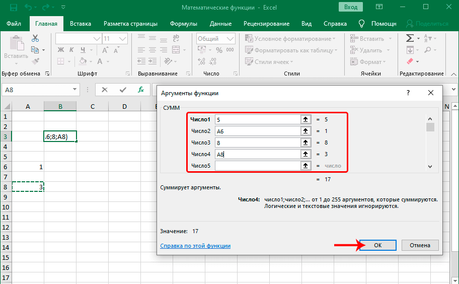
SUMMESLI
Using the formulas in which this function is written, the user can calculate the sum of values that meet certain conditions. They will help automate the selection of values that fit specific criteria. The formula looks like this: =SUMIF(Range, Criteria, Sum_Range). We see that several parameters are given as parameters of this function:
- Cell range. This includes those cells that should be checked against the condition specified in the second argument.
- Condition. The condition itself, against which the range specified in the first argument will be checked. Possible conditions are as follows: greater than (sign >), less than (sign <), not equal (<>).
- summation range. The range that will be summed up if the first argument matches the condition. The range of cells and summation can be the same.
The third argument is optional.
Function PRIVATE
Typically, users use the standard formula for dividing two or more numbers. The sign / is used to perform this arithmetic operation. The disadvantage of this approach is the same as with manual execution of any other arithmetic operations. If the amount of data is too large, it is quite difficult to calculate them correctly. You can automate the division process using the function PRIVATE. Its syntax is the following: =PARTIAL(Numerator, Denominator). As you can see, we have two main arguments here: the numerator and the denominator. They correspond to the classical arithmetic numerator and denominator.
Function PRODUCT
This is the opposite of the previous function, which performs the multiplication of numbers or ranges that are entered there as arguments. In the same way as in previous similar functions, this makes it possible to enter information not only about specific numbers, but also ranges with numerical values.
Function ROUNDWOOD
Rounding is one of the most popular actions in various areas of human life. And although after the introduction of computer technology it is not as necessary as before, this formula is still used to bring the number into a beautiful form that does not contain a large number of decimal places. Below you can see what the generic syntax for a formula using this function looks like: =ROUND(number,number_digits). We see that there are two arguments here: the number that will be roundable and the number of digits that will be visible in the end. 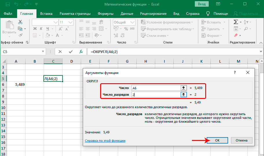
Rounding is a great opportunity to make life easier for the spreadsheet reader if precision isn’t critical. Absolutely any routine task allows the use of rounding, since in everyday situations it is very rare to engage in activities where you need to carry out calculations with an accuracy of one hundred thousandth of a number. This function rounds a number according to standard rules,
Function POWER
Beginning Excel users very often wonder how to raise a number to a power. For this, a simple formula is used, which automatically multiplies the number by itself a certain number of times. Contains two required arguments: =POWER(number, power). As you can see from the syntax, the first argument allows you to specify a number that will be multiplied a certain number of times. The second argument is the degree to which it will be raised. 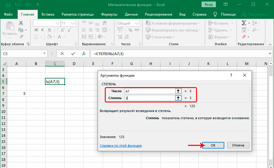
Function ROOT
This function allows you to determine the square root of the value given in parentheses. The formula template looks like this: =ROOT(number). If you enter this formula through its input box, you will see that there is only one argument to be entered.
Function LOG
This is another mathematical function that allows you to calculate the logarithm of a certain number. It takes two arguments to make it work: a number and the base of the logarithm. The second argument is, in principle, optional. In this case, the value will take the one that is programmed in Excel as the one that is specified by default. That is, 10.
By the way, if you need to calculate the decimal logarithm, you can use the LOG10 function.
Function RESIDUE
If you can’t divide one number by another so that the result is an integer, then you often have to get the remainder. To do this, you need to enter the formula =REMAID(number, divisor). We see that there are two arguments. The first is the number on which the division operation is performed. The second is the divisor, the value by which the number is divisible. You can enter this formula either by putting the appropriate values in brackets when entering it manually, or through the function entry wizard.
An interesting fact: the operation of division with a remainder is also called integer division and is a separate category in mathematics. It is also often referred to as modulo division. But in practice, such a term is best avoided, because confusion in terminology is possible.
Less popular math functions
Some features are not so popular, but they still gained wide acceptance. First of all, this is a function that allows you to select a random number in a certain corridor, as well as one that makes a Roman number out of an Arabic number. Let’s look at them in more detail.
Function BETWEEN THE CASE
This function is interesting in that it displays any number that is between the value A and the value B. They are also its arguments. The value A is the lower limit of the sample, and the value B is the upper limit.
There are no completely random numbers. All of them are formed according to certain patterns. But this does not affect the practical use of this formula, just an interesting fact.
Function ROMAN
The standard number format used in Excel is Arabic. But you can also display numbers in Roman format. To do this, you can use a special function that has two arguments. The first one is a reference to the cell containing the number, or the number itself. The second argument is the form.
Despite the fact that Roman numbers are no longer as common as they used to be, they are still sometimes used in . In particular, this form of representation is necessary in such cases:
- If you need to record a century or a millennium. In this case, the recording form is as follows: XXI century or II millennium.
- Conjugation of verbs.
- Если было несколько монархов с одним именем, то римское число обозначает его порядковый номер.
- Corps designation in the Armed Forces.
- On a military uniform in the Armed Forces, the blood type is recorded using Roman numerals so that a wounded unknown soldier can be saved.
- Sheet numbers are also often displayed in Roman numerals so that references within the text do not need to be corrected if the preface changes.
- To create a special marking of the dials in order to add a rarity effect.
- Designation of the serial number of an important phenomenon, law or event. For example, World War II.
- In chemistry, Roman numerals denote the ability of chemical elements to create a certain number of bonds with other elements.
- In solfeggio (this is a discipline that studies the structure of the musical range and develops an ear for music), Roman numerals indicate the number of the step in the sound range.
Roman numerals are also used in calculus to write the number of the derivative. Thus, the range of application of Roman numerals is huge.
Сейчас почти не используются те форматы даты, которые подразумевают запись в виде римских цифр, но подобный способ отображения был довольно популярен в докомпьютерную эпоху. Ситуации, в которых используются римские цифры, могут отличаться в разных странах. Например, в Литве они активно используются на дорожных знаках, для обозначения дней недели, а также на витринах.
Time for some summing up. Excel formulas are a great opportunity to make your life easier. Today we have given the TOP of the most popular mathematical functions in spreadsheets that allow you to cover most of the tasks. But for solving specific problems, special formulas are better suited.