Contents
Yesterday in the marathon 30 Excel functions in 30 days we found text strings using the function SEARCH (SEARCH) and also used IFERROR (IFERROR) and ISNUMBER (ISNUMBER) in situations where the function throws an error.
On the 19th day of our marathon, we will study the function MATCH (SEARCH). It looks up a value in an array and, if a value is found, returns its position.
So, let’s turn to the reference information on the function MATCH (MATCH) and look at a few examples. If you have your own examples or approaches for working with this function, please share them in the comments.
Function 19: MATCH
Function MATCH (MATCH) returns the position of a value in an array, or an error #AT (#N/A) if not found. An array can be either sorted or unsorted. Function MATCH (MATCH) is not case sensitive.
How can you use the MATCH function?
Function MATCH (MATCH) returns the position of an element in an array, and this result can be used by other functions such as INDEX (INDEX) or VLOOKUP (VPR). For example:
- Find the position of an element in an unsorted list.
- Use with CHOOSE (SELECT) to convert student performance to letter grades.
- Use with VLOOKUP (VLOOKUP) for flexible column selection.
- Use with INDEX (INDEX) to find the nearest value.
Syntax MATCH
Function MATCH (MATCH) has the following syntax:
MATCH(lookup_value,lookup_array,[match_type])
ПОИСКПОЗ(искомое_значение;просматриваемый_массив;[тип_сопоставления])
- lookup_value (lookup_value) – Can be text, number, or boolean.
- lookup_array (lookup_array) – an array or array reference (adjacent cells in the same column or same row).
- match_type (match_type) can take three values: -1, 0 or 1. If the argument is omitted, it is equivalent to 1.
Traps MATCH (MATCH)
Function MATCH (MATCH) returns the position of the found element, but not its value. If you want to return a value, use MATCH (MATCH) together with the function INDEX (INDEX).
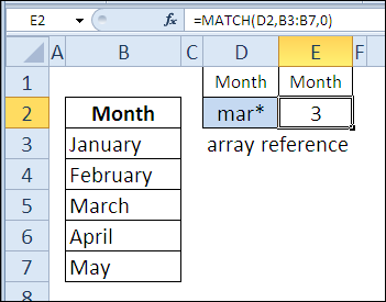
Example 1: Finding an element in an unsorted list
For an unsorted list, you can use 0 as argument value match_type (match_type) to search for an exact match. If you want to find an exact match of a text string, you can use wildcard characters in the search value.
In the following example, to find the position of a month in a list, we can write the name of the month, either in whole or in part, using wildcards.
=MATCH(D2,B3:B7,0)
=ПОИСКПОЗ(D2;B3:B7;0)
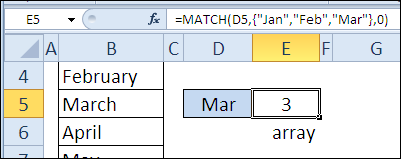
As an argument lookup_array (lookup_array) you can use an array of constants. In the following example, the desired month is entered in cell D5, and the names of the months are substituted as the second argument to the function MATCH (MATCH) as an array of constants. If you enter a later month in cell D5, for example, Oct (October), then the result of the function will be #AT (#N/A).
=MATCH(D5,{"Jan","Feb","Mar"},0)
=ПОИСКПОЗ(D5;{"Jan";"Feb";"Mar"};0)
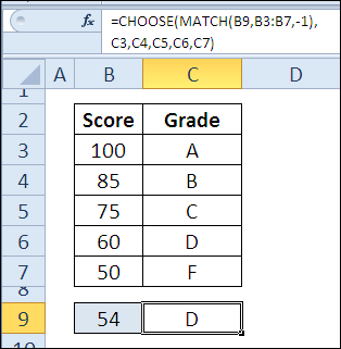
Example 2: Change student grades from percentages to letters
You can convert student grades to a letter system using the function MATCH (MATCH) just like you did with VLOOKUP (VPR). In this example, the function is used in conjunction with CHOOSE (CHOICE), which returns the estimate we need. Argument match_type (match_type) is set equal to -1, because the scores in the table are sorted in descending order.
When the argument match_type (match_type) is -1, the result is the smallest value that is greater than or equivalent to the desired value. In our example, the desired value is 54. Since there is no such value in the list of scores, the element corresponding to the value 60 is returned. Since 60 is in fourth place in the list, the result of the function CHOOSE (SELECT) will be the value that is in the 4th position, i.e. cell C6, which contains the score D.
=CHOOSE(MATCH(B9,B3:B7,-1),C3,C4,C5,C6,C7)
=ВЫБОР(ПОИСКПОЗ(B9;B3:B7;-1);C3;C4;C5;C6;C7)
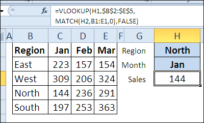
Example 3: Create a flexible column selection for VLOOKUP (VLOOKUP)
To give more flexibility to the function VLOOKUP (VLOOKUP) You can use MATCH (MATCH) to find the column number, rather than hard-coding its value into the function. In the following example, users can select a region in cell H1, this is the value they are looking for VLOOKUP (VPR). Next, they can select a month in cell H2, and the function MATCH (MATCH) will return the column number corresponding to that month.
=VLOOKUP(H1,$B$2:$E$5,MATCH(H2,B1:E1,0),FALSE)
=ВПР(H1;$B$2:$E$5;ПОИСКПОЗ(H2;B1:E1;0);ЛОЖЬ)
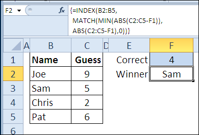
Example 4: Finding the nearest value using INDEX (INDEX)
Function MATCH (MATCH) works great in combination with the function INDEX (INDEX), which we will look at more closely a little later in this marathon. In this example, the function MATCH (MATCH) is used to find the nearest to the correct number from several guessed numbers.
- Function ABS returns the modulus of the difference between each guessed and correct number.
- Function MIN (MIN) finds the smallest difference.
- Function MATCH (MATCH) finds the address of the smallest difference in the list of differences. If there are multiple matching values in the list, the first one will be returned.
- Function INDEX (INDEX) returns the name corresponding to this position from the list of names.
=INDEX(B2:B5,MATCH(MIN(ABS(C2:C5-F1)),ABS(C2:C5-F1),0))
=ИНДЕКС(B2:B5;ПОИСКПОЗ(МИН(ABS(C2:C5-F1));ABS(C2:C5-F1);0))