


Contents
More and more often I meet in the reporting of different companies and hear requests from trainees to explain how a cascade diagram of deviations is built – it is also a “waterfall”, it is also a “waterfall”, it is also a “bridge”, it is also a “bridge”, etc. . It looks something like this:

From a distance, it really looks like a cascade of waterfalls on a mountain river or a hanging bridge – who sees what 🙂
The peculiarity of such a diagram is that:
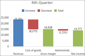
- We clearly see the initial and final value of the parameter (the first and last columns).
- Positive changes (growth) are displayed in one color (usually green), and negative ones (decline) to others (usually red).
- Sometimes the chart may also contain subtotal columns (graylanded on the x-axis columns).
In everyday life, such diagrams are usually used in the following cases:
- Visual dynamics display any process in time: cash flow (cash-flow), investments (we invest in a project and get profit from it).
- Visualization plan implementation (the leftmost column in the diagram is a fact, the rightmost column is a plan, the entire diagram reflects our process of moving towards the desired result)
- When you need visual show factorsthat affect our parameter (factorial analysis of profit – what it consists of).
There are several ways to build such a chart – it all depends on your version of Microsoft Excel.
Method 1: Easiest: Built-in type in Excel 2016 and newer
If you have Excel 2016, 2019 or later (or Office 365), then building such a chart is not difficult – these versions of Excel already have this type built in by default. It will only be necessary to select a table with data and select on the tab Insert (Insert) Command cascading (Waterfall):

As a result, we will get an almost ready-made diagram:

You can immediately set the desired fill colors for the positive and negative columns. The easiest way to do this is to select the appropriate rows Increase и decrease directly in the legend and by right-clicking on them, select the command Fill (Fill):

If you need to add columns with subtotals or a final column-total to the chart, then it is most convenient to do this using functions SUBTOTALS (SUBTOTALS) or UNIT (AGGREGATE). They will calculate the amount accumulated from the beginning of the table, while excluding from it the similar totals located above:

In this case, the first argument (9) is the code of the mathematical summation operation, and the second (0) causes the function to ignore already calculated totals for previous quarters in the results.
After adding rows with totals, it remains to select the total columns that have appeared on the diagram (make two consecutive single clicks on the column) and, by right-clicking on the mouse, select the command Set as total (Set as total):

The selected column will land on the x-axis and automatically change color to gray.
That, in fact, is all – the waterfall diagram is ready:

Method 2. Universal: invisible columns
If you have Excel 2013 or older versions (2010, 2007, etc.), then the method described above will not work for you. You will have to go around and cut out the missing waterfall chart from a regular stacked histogram (summing the bars on top of each other).
The trick here is to use transparent prop columns to raise our red and green data rows to the correct height:

To build such a chart, we need to add a few more auxiliary columns with formulas to the source data:

- First, we need to split our original column by separating the positive and negative values into separate columns using the function IF (IF).
- Secondly, you will need to add a column in front of the columns pacifiers, where the first value will be 0, and starting from the second cell, the formula will calculate the height of those very transparent supporting columns.
After that, it remains to select the entire table except for the original column Flow and create a regular stacked histogram across Inset — Histogram (Insert — Column Chart):

If you now select the blue columns and make them invisible (right-click on them – Row Format – Fill – No Fill), then we just get what we need.
The advantage of this method is simplicity. In the minuses – the need to count auxiliary columns.
Method 3. If we go into the red, everything is more difficult
Unfortunately, the previous method only works adequately for positive values. If at least in some area our waterfall goes into a negative area, then the complexity of the task increases significantly. In this case, it will be necessary to calculate each row (dummy, green and red) separately for the negative and positive parts with formulas:

In order not to suffer much and not to reinvent the wheel, a ready-made template for such a case can be downloaded in the title of this article.
Method 4. Exotic: up-down bands
This method is based on the use of a special little-known element of flat charts (histograms and graphs) – Up-down bands (Up-Down Bars). These bands connect the points of two graphs in pairs to clearly show which of the two points is higher or lower, which is actively used when visualizing the plan-fact:

It is easy to figure out that if we remove the lines of the charts and leave only the up-down bands on the chart, then we will get the same “waterfall”.
For such a construction, we need to add two more additional columns to our table with simple formulas that will calculate the position of the two required invisible graphs:

To create a “waterfall”, you need to select a column with months (for signatures along the X axis) and two additional columns Schedule 1 и Schedule 2 and build a regular graph for starters using Insert – Graph (Insert — Line Сhart):

Now let’s add up-down bands to our chart:
- In Excel 2013 and newer, this must be selected on the tab Constructor Command Add Chart Element — Bands of increase-decrease (Design — Add Chart Element — Up-Down Bars)
- In Excel 2007-2010 – go to tab Layout – Advance-Decrement Bars (Layout — Up-Down Bars)
The chart will then look something like this:

It remains to select the graphs and make them transparent by clicking on them in turn with the right mouse button and selecting the command Data series format (Format series). Similarly, you can change the standard, rather shabby looking black and white stripe colors to green and red to get a nicer picture in the end:

In the latest versions of Microsoft Excel, the width of the bars can be changed by clicking on one of the transparent graphs (not the bars!) with the right mouse button and selecting the command Data Series Format – Side Clearance (Format series — Gap width).
In older versions of Excel, you had to use the Visual Basic command to fix this:
- Highlight the built diagram
- Press the keyboard shortcut Alt+F11to get into the Visual Basic Editor
- Press keyboard shortcut Ctrl+Gto open the direct command input and debug panel immediate (usually located at the bottom).
- Copy and paste the following command there: ActiveChart.ChartGroups(1).GapWidth = 30 and press Enter:

You can, of course, play around with the parameter value if you wish. GapWidthto achieve the desired clearance:

- How to build a bullet chart in Excel to visualize KPI
- What’s New in Charts in Excel 2013
- How to create an interactive “live” chart in Excel