


Contents
In this article, you’ll find two quick ways to change the color of a cell based on its value in Excel 2013, 2010, and 2007. Also, you’ll learn how to use formulas in Excel to change the color of empty cells or cells with formula errors.
Everyone knows that to change the fill color of a single cell or an entire range in Excel, just click the button Fill color (Fill color). But what if you need to change the fill color of all cells containing a certain value? Moreover, what if you want the fill color of each cell to change automatically as the contents of that cell change? Further in the article you will find answers to these questions and get a couple of useful tips that will help you choose the right method for solving each specific problem.
How to dynamically change the color of a cell in Excel based on its value
The fill color will change depending on the value of the cell.
Problem: You have a table or range of data and you want to change the fill color of cells based on their values. Moreover, it is necessary that this color change dynamically, reflecting changes in the data in the cells.
Decision: Use conditional formatting in Excel to highlight values greater than X, less than Y, or between X and Y.
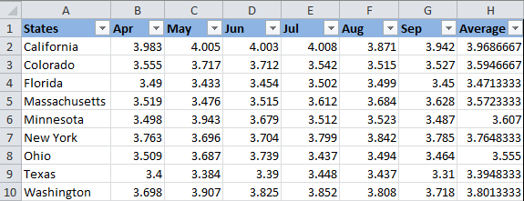
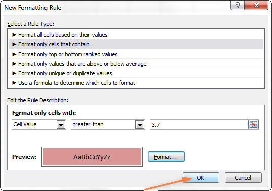
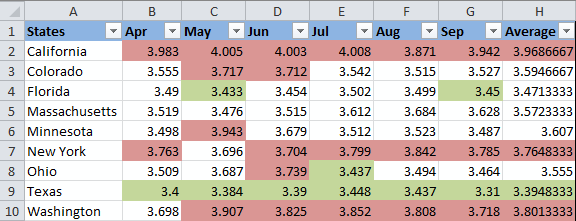
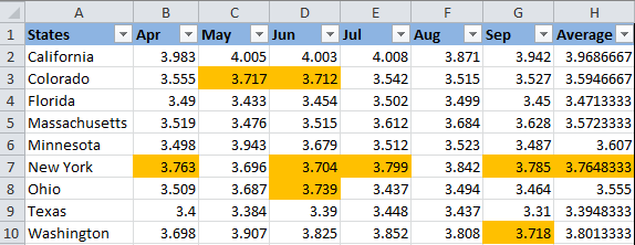
Let’s say you have a list of gas prices in different states, and you want prices that are higher than $ 3.7, were highlighted in red, and smaller or equal $ 3.45 – green.
Note: The screenshots for this example were taken in Excel 2010, however, in Excel 2007 and 2013, the buttons, dialogs, and settings will be exactly the same or slightly different.
So, here’s what you need to do step by step:
- Select the table or range in which you want to change the cell fill color. In this example, we highlight $B$2:$H$10 (column headings and the first column containing the names of the states are not selected).
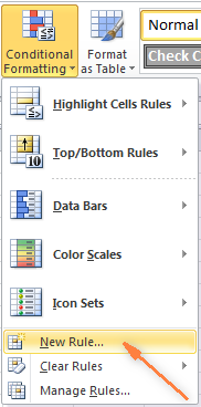
- Click the Home (Home), in the section Styles (Styles) click Conditional Formatting (Conditional Formatting) > New Rules (Create a rule).

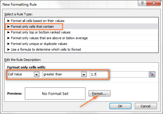
- At the top of the dialog box New Formatting Rule (Create Formatting Rule) in the field Select a Rule Type (Select rule type) select Format only cells that contain (Format only cells that contain).
- At the bottom of the dialog box in the box Format Only Cells with (Format only cells that meet the following condition) Set the conditions for the rule. We choose to format only cells with the condition: Cell Value (cell value) – greater than (more) – 3.7as shown in the figure below.Then press the button Size (Format) to select which fill color should be applied if the specified condition is met.
- In the dialog box that appears Format Cells (Format Cells) tab Fill (Fill) and choose a color (we chose reddish) and click OK.
- After that you will return to the window New Formatting Rule (Creating a formatting rule) where in the field Preview (Sample) will show a sample of your formatting. If you are satisfied, click OK.
 Then press the button Size (Format) to select which fill color should be applied if the specified condition is met.
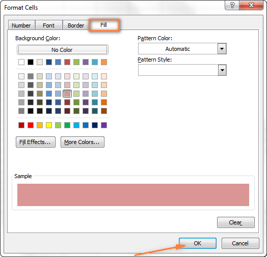
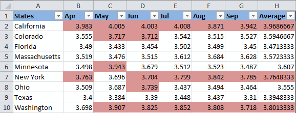
The result of your formatting settings will look something like this:
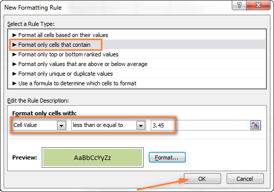
Since we need to set up another condition that allows us to change the fill color to green for cells with values less than or equal to 3.45, then press the button again New Rules (Create Rule) and repeat steps 3 to 6, setting the desired rule. Below is a sample of the second conditional formatting rule we created:
When everything is ready – click OK. You now have a nicely formatted table that allows you to see the maximum and minimum gas prices in different states at a glance. Good for them there, in Texas! 🙂
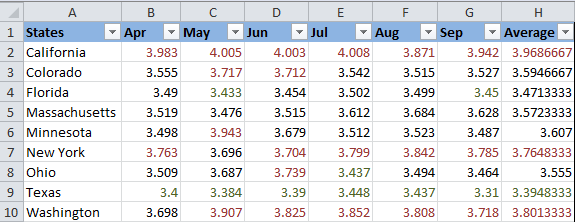
Tip: In the same way, you can change the font color depending on the value of the cell. To do this, just open the tab Font (Font) in the dialog box Format Cells (Cell Format) as we did in step 5 and select the desired font color.
How to set a constant cell color based on its current value
Once set, the fill color will not change, no matter how the contents of the cell change in the future.
Problem: You want to adjust the color of a cell based on its current value, and you want the fill color to stay the same even when the cell’s value changes.
Decision: Find all cells with a specific value (or values) using the tool Find All (Find All) and then change the format of the found cells using the dialog box Format Cells (cell format).
This is one of those rare tasks for which there is no explanation in the Excel help files, forums or blogs, and for which there is no direct solution. And this is understandable, since this task is not typical. And yet, if you need to change the cell fill color permanently, that is, once and for all (or until you change it manually), follow these steps.
Find and select all cells that meet a given condition
Several scenarios are possible here, depending on what type of value you are looking for.
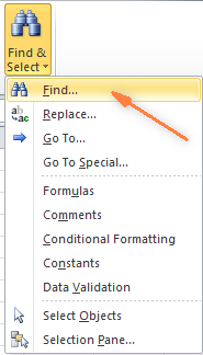
If you want to color cells with a specific value, for example, 50, 100 or 3.4 – then on the tab Home (Home) in the section Editing (Editing) click Find Select (Find and highlight) > Find (Find).
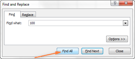
Enter the desired value and click Find All (Find all).
Tip: On the right side of the dialog box Find and Replace (Find and Replace) there is a button Options (Options), by pressing which you will have access to a number of advanced search settings, such as Match Case (case sensitive) and Match entire cell content (Entire cell). You can use wildcard characters such as the asterisk (*) to match any string of characters, or the question mark (?) to match any single character.
Regarding the previous example, if we need to find all gasoline prices from 3.7 to 3.799, then we will set the following search criteria:
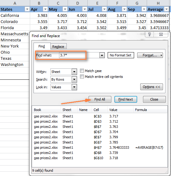
Now click on any of the found items at the bottom of the dialog box Find and Replace (Find and Replace) and click Ctrl + Ato highlight all found entries. After that press the button Fermer (Close).
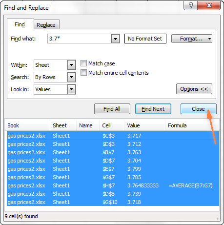
This is how you can select all cells with a given value (values) using the option Find All (Find All) in Excel.
However, in reality, we need to find all gasoline prices that exceed $ 3.7. Unfortunately the tool Find and Replace (Find and Replace) cannot help us with this.
Change the Fill Colors of Selected Cells Using the Format Cells Dialog Box
You now have all the cells with the given value (or values) selected, we just did this with the tool Find and Replace (Find and replace). All you have to do is set the fill color for the selected cells.
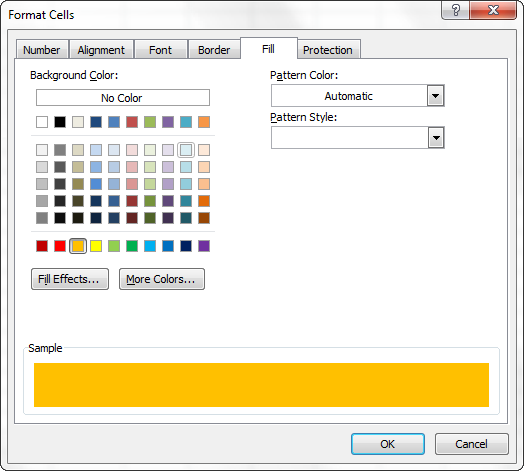
Open a dialog box Format Cells (Cell Format) in any of 3 ways:
- pressing Ctrl + 1.
- by clicking on any selected cell with the right mouse button and selecting the item from the context menu Format Cells (cell format).
- tab Home (Home) > Cells. Cells. (cells) > Size (Format) > Format Cells (cell format).
Next, adjust the formatting options as you like. This time we’ll set the fill color to orange, just for a change 🙂
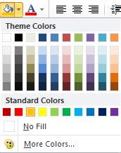
If you want to change only the fill color without touching the rest of the formatting options, you can simply click the button Fill color (Fill color) and choose the color you like.
Here is the result of our formatting changes in Excel:
Unlike the previous method (with conditional formatting), the fill color set in this way will never change itself without your knowledge, no matter how the values change.
Change the fill color for special cells (empty, with an error in the formula)
As in the previous example, you can change the fill color of specific cells in two ways: dynamically and statically.
Use a formula to change the fill color of special cells in Excel
The cell color will change automatically depending on the value of the cell.
You will most likely use this method of solving the problem in 99% of cases, that is, the filling of the cells will change in accordance with the condition you specified.
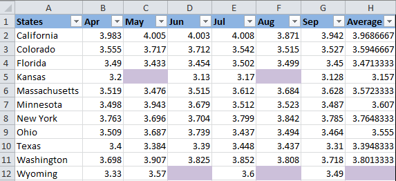
For example, let’s take the gasoline price table again, but this time we will add a couple more states, and make some cells empty. Now see how you can find these empty cells and change their fill color.
- On the Advanced tab Home (Home) in the section Styles (Styles) click Conditional Formatting (Conditional Formatting) > New Rules (Create a rule). Just like in the 2nd step of the example How to dynamically change the color of a cell based on its value.
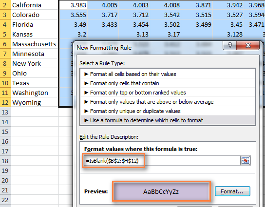
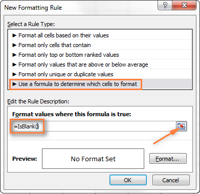
- In the dialog box New Formatting Rule (Create a formatting rule) select an option Use a formula to determine which cells to format (Use a formula to determine which cells to format). Further into the field Format values where this formula is true (Format values for which the following formula is true) enter one of the formulas:
- to change the fill of empty cells
=ISBLANK()=ЕПУСТО() - to change the shading of cells containing formulas that return an error
=ISERROR()=ЕОШИБКА()
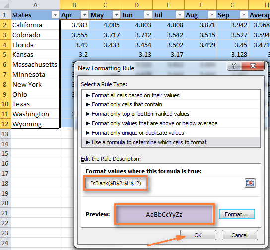
Since we want to change the color of empty cells, we need the first function. Enter it, then place the cursor between the brackets and click the range selection icon on the right side of the line (or type the desired range manually):
=ISBLANK(B2:H12)=ЕПУСТО(B2:H12) - to change the fill of empty cells
- Нажмите кнопку Size (Format), select the desired fill color on the tab Fill (Fill), and then click OK. Detailed instructions are given in step 5 of the example “How to dynamically change the color of a cell based on its value.” A sample of the conditional formatting you set up will look something like this:
- If you are happy with the color, click OK. You will see how the created rule will be immediately applied to the table.
Change the fill color of special cells statically
Once configured, the fill will remain unchanged, regardless of the value of the cell.
If you want to set a permanent fill color for empty cells or cells with formulas that contain errors, use this method:
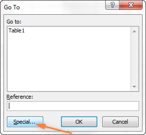
- Select a table or range and click F5to open the dialog Go To (Jump), then press the button Special (Highlight).
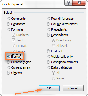
- In the dialog box Go to Special (Select a group of cells) check the option blanks (Blank Cells) to select all empty cells.If you want to highlight cells containing formulas with errors, check the option Formulas (formulas) > Errors (Mistakes). As you can see in the picture above, there are many other settings available to you.
- Finally, change the fill of the selected cells or set any other formatting options using the dialog box Format Cells (Format Cells), as described in Changing the Fill of Selected Cells.
 If you want to highlight cells containing formulas with errors, check the option Formulas (formulas) > Errors (Mistakes). As you can see in the picture above, there are many other settings available to you.
Do not forget that formatting settings made in this way will be preserved even when empty cells are filled with values or mistakes in formulas are corrected. It’s hard to imagine that someone might need to go this way, except for the purposes of the experiment 🙂